| Box | Contents | Probabilities | H |
|---|---|---|---|
| Box 1 | {A,A,A,A} | (1) | 0 |
| Box 2 | {A,A,B,B} | (½, ½) | 1 |
| Box 3 | {A,B,C,D} | (¼,¼,¼,¼) | 2 |
| Box 4 | {A,A,B,C} | (½,¼,¼) | 1.5 |
Information Theory
Quantifying Uncertainty and Information
EDA for Machine Learning
A Coda to Part 1
Part 1 introduced EDA from a geometric perspective:
- Scatter plots and conditional distributions
- Clustering of observations
- Simulation
This chapter takes a different approach: information theory.
These concepts appear repeatedly in ML:
- Decision tree construction
- Neural network training (cross-entropy loss)
- Model comparison
Chapter Roadmap
| Concept | Intuition |
|---|---|
| Entropy | How uncertain is an outcome? |
| Mutual Information | How much information do (X, Y) share? |
| KL Divergence | How costly is using the wrong distribution? |
All three connect to the Twenty Questions game.
Entropy
Entropy: The Yes-No Questions Game
Imagine a box of tickets, each bearing a capital letter.
The game:
- You are shown the box of tickets.
- A ticket is drawn at random, but you can’t see it.
- You ask yes-no questions until you can identify the letter with certainty.
- Goal: minimize average number of questions.
Entropy measures the difficulty of this game.
Box 1: No Uncertainty
\[\text{Box 1: } \{A, A, A, A\}\]
How many questions needed?
Zero. You already know the answer.
\[H = 0\]
Box 2: One Bit of Uncertainty
\[\text{Box 2: } \{A, A, B, B\}\]
One question: “Is it A?”
One question always suffices.
\[H = 1 \text{ bit}\]
Box 3: Two Bits of Uncertainty
\[\text{Box 3: } \{A, B, C, D\}\]
First question: “Is it A or B?”
Second question: “Is it [first of the pair]?”
Two questions always suffices.
\[H = 2 \text{ bits}\]
Box 4: Fractional Entropy
\[\text{Box 4: } \{A, A, B, C\}\]
Optimal strategy:
- First ask: “Is it A?” (probability ½)
- If yes → done (1 question)
- If no → one more question to distinguish B from C
\[\text{Average} = \frac{1}{2}(1) + \frac{1}{2}(2) = \frac{3}{2} \text{ questions}\]
\[H = 1.5 \text{ bits}\]
The Entropy Formula
For a probability distribution \((p_1, p_2, \ldots, p_K)\):
\[H = -\sum_{k=1}^{K} p_k \log_2(p_k)\]
Equivalently:
\[H = \sum_{k=1}^{K} p_k \log_2\left(\frac{1}{p_k}\right)\]
Units: bits (binary digits) when using \(\log_2\)
Entropy Examples
Pattern: Entropy is maximized when all outcomes are equally likely.
Binary Search Strategy
General approach:
- Partition tickets into two groups of equal (or nearly equal) probability
- Ask which group contains the drawn ticket
- Repeat within the identified group
Maximum questions: \(\lceil \log_2(K) \rceil\) for \(K\) distinct values
Average questions: Often fewer (as Box 4 shows)
Mutual Information
Joint Entropy: Two Variables
Now each ticket has a letter and a number.
\[\text{Box 5: } \{A_1, A_1, B_1, C_1, A_2, A_2, B_2, C_2\}\]
This is equivalent to:
- Draw letter from \(\{A, A, B, C\}\) → \(H_{\text{letter}} = 1.5\)
- Draw number from \(\{1, 2\}\) → \(H_{\text{number}} = 1\)
Independently!
Entropy of Independent Variables
When \(X\) and \(Y\) are independent:
\[H_{X,Y} = H_X + H_Y\]
For Box 5:
\[H = 1.5 + 1 = 2.5 \text{ bits}\]
Intuition: No information about the letter helps you guess the number, and vice versa.
Mutual Information: When Variables Are Dependent
\[\text{Box 6: } \{A_1, A_2, B_1, C_2\}\]
Same marginal distributions:
- Letters: \(\{A, A, B, C\}\) → \(H_{\text{letter}} = 1.5\)
- Numbers: \(\{1, 1, 2, 2\}\) → \(H_{\text{number}} = 1\)
But now they’re dependent!
The Power of Dependence
New strategy for Box 6:
- First ask: “Is the number 1?” (1 question)
- If yes → letter is A or B (1 more question)
- If no → letter is A or C (1 more question)
Total: 2 questions (not 2.5!)
\[H_{X,Y} = 2 < H_X + H_Y = 2.5\]
Mutual Information Defined
\[MI_{X,Y} = H_X + H_Y - H_{X,Y}\]
Interpretation: The reduction in uncertainty about \(Y\) from knowing \(X\) (and vice versa).
For Box 6:
\[MI = 1.5 + 1 - 2 = 0.5 \text{ bits}\]
Properties:
- \(MI \geq 0\) always
- \(MI = 0\) if and only if \(X\) and \(Y\) are independent
Mutual Information: Visual Intuition
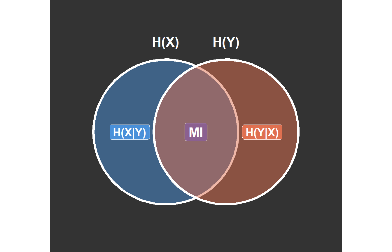
Figure 1
\[H_{X,Y} = H_X + H_Y - MI_{X,Y}\]
KL Divergence
KL Divergence: The Cost of Being Wrong
Scenario: You’re shown Box 5 (independent) and optimized your strategy accordingly, but the actual box is Box 6 (dependent).
- Your strategy expects 2.5 questions on average
- Optimal for Box 6 needs only 2 questions
The cost of misinformation: 0.5 extra questions per round
KL Divergence Defined
\[KL(P \| Q) = \sum_{x} P(x) \log_2\left(\frac{P(x)}{Q(x)}\right)\]
Interpretation: Expected extra bits needed when using code optimized for \(Q\) but the true distribution is \(P\).
\(P\) = true distribution (what the box actually is)
\(Q\) = assumed distribution (what you think it is)
KL Divergence Example
| x | P(x) | Q(x) | log₂(P/Q) | Term |
|---|---|---|---|---|
| A₁ | 1/4 | 1/4 | 0 | 0 |
| A₂ | 1/4 | 1/4 | 0 | 0 |
| B₁ | 1/4 | 1/8 | 1 | 1/4 |
| B₂ | 0 | 1/8 | — | 0 |
| C₁ | 0 | 1/8 | — | 0 |
| C₂ | 1/4 | 1/8 | 1 | 1/4 |
\[KL(P \| Q) = 0 + 0 + \frac{1}{4} + 0 + 0 + \frac{1}{4} = \frac{1}{2}\]
Confirms: Using the wrong distribution costs 0.5 bits.
KL Divergence Properties
Not symmetric: \(KL(P \| Q) \neq KL(Q \| P)\) in general
Non-negative: \(KL(P \| Q) \geq 0\)
Zero iff identical: \(KL(P \| Q) = 0 \Leftrightarrow P = Q\)
Not a true distance (fails triangle inequality)—hence “divergence”
ML Applications
Where These Ideas Appear in ML
| Concept | ML Application |
|---|---|
| Entropy | Decision tree splits |
| Mutual Information | Feature selection |
| KL Divergence | Loss functions, variational inference1 |
| Cross-entropy | Classification loss |
Cross-Entropy Loss
The standard loss function for classification—cross-entropy—is derived from KL divergence.
Minimizing cross-entropy loss is equivalent to minimizing the divergence between:
- the model’s predicted probabilities
- the observed outcomes
Decision Trees and Information Gain
When splitting a node:
\[\text{Information Gain} = H(\text{parent}) - \sum_{\text{children}} \frac{n_{\text{child}}}{n_{\text{parent}}} H(\text{child})\]
Strategy: Choose the split that maximizes information gain.
Feature Selection with Mutual Information
Correlation captures linear relationships.
Mutual Information captures any dependence.
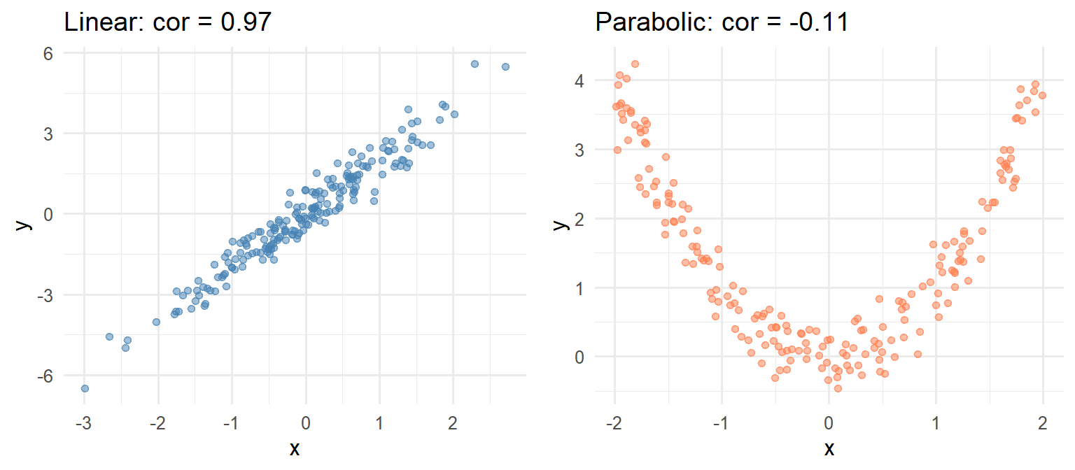
Correlation misses the parabolic relationship. Mutual information catches it.
Summary
Summary: Three Linked Concepts
| Concept | Question Answered |
|---|---|
| Entropy \(H\) | How uncertain is \(X\)? |
| Mutual Information \(MI\) | How much does \(X\) tell us about \(Y\)? |
| KL Divergence \(KL\) | How costly is assuming \(Q\) when truth is \(P\)? |
\[MI_{X,Y} = KL\big(P_{X,Y} \| P_X \cdot P_Y\big)\]
Mutual information is the KL divergence from independence.
Key Formulas
\[H(X) = -\sum_x P(x) \log_2 P(x)\]
\[MI_{X,Y} = H_X + H_Y - H_{X,Y}\]
\[KL(P \| Q) = \sum_x P(x) \log_2 \frac{P(x)}{Q(x)}\]
Exercises
Team Exercise 1: Entropy of a Fair Die
- Calculate the entropy \(H\) for a fair six-sided die.
- Compare to a loaded die with \(P(6) = 0.5\) and others equal.
- Which has higher entropy? Why does this make sense?
- Generalize: what is \(H\) for a discrete uniform distribution on \(K\) outcomes?
Team Exercise 2: UCB Admissions Revisited
Consider a box of tickets matching the UC Berkeley admissions data.
- Restricting to just “Admitted” vs. “Rejected,” calculate \(H_{\text{decision}}\).
- Now calculate the joint entropy \(H_{\text{decision, sex}}\) and mutual information \(MI\).
- What does \(MI \approx 0\) tell us about marginal sex bias?
- How would you incorporate department to reveal Simpson’s paradox?
Team Exercise 3: Cross-Entropy Loss
A classifier predicts probabilities for 3 classes. True class is 1.
Compare cross-entropy loss for these predictions:
| Prediction | \((\hat{p}_1, \hat{p}_2, \hat{p}_3)\) |
|---|---|
| Confident & correct | \((0.9, 0.05, 0.05)\) |
| Less confident | \((0.6, 0.2, 0.2)\) |
| Uniform | \((0.33, 0.33, 0.34)\) |
- Calculate the loss for each.
- What happens as \(\hat{p}_1 \to 0\)?
- Why is this the standard loss for classification?
Discussion Questions
When would mutual information identify a useful feature that correlation misses?
Why is KL divergence not symmetric? Give an example where direction matters.
How does information theory connect to compression?
Resources
A Mathematical Theory of Communication — Shannon’s original 1948 paper
Shannon Entropy, Information Gain, and Picking Balls from Buckets — Udacity tutorial
Mutual Information — Wikipedia
Cross-entropy — Wikipedia
Information gain in decision trees — Wikipedia