| father | mother | child | gender |
|---|---|---|---|
| 78.5 | 67.0 | 73.2 | male |
| 75.5 | 66.5 | 73.5 | male |
| 75.0 | 64.0 | 71.0 | male |
| 75.0 | 64.0 | 70.5 | male |
| 75.0 | 58.5 | 72.0 | male |
| 74.0 | 68.0 | 69.5 | female |
Linear Regression
Projection onto Feature Space
EDA for Machine Learning
The Big Picture
Linear Algebra Meets Statistics
In Part 1, we explored data through:
- Scatter plots and conditional distributions
- Clustering observations
- Simulation
Part 2 takes a different approach: the geometry of linear algebra.
Core insight
Least-squares regression is orthogonal projection onto feature space.
Why Geometry?
Linear algebra provides:
- A unified language for regression, PCA, and classification
- Geometric intuition for what “fitting” means
- Tools that scale to high dimensions
This chapter: Regression as projection
Next chapters: PCA and LDA as finding optimal subspaces
Two Perspectives on Data
| Perspective | Focus | Visualization |
|---|---|---|
| Row | Observations as points | Scatter plots in feature space |
| Column | Features as vectors | Vectors in observation space |
Most visualizations use the row perspective.
Most linear algebra uses the column perspective.
Understanding both is essential.
Data Example: Family Heights
Galton’s Height Data
In 1885, Francis Galton studied heights of parents and children.
- 205 families (oldest child only)
- 179 sons, 26 daughters
- Variables: father’s height, mother’s height, child’s height
The Data Matrix
Goal: Predict child’s height from parents’ heights.
3D Visualization
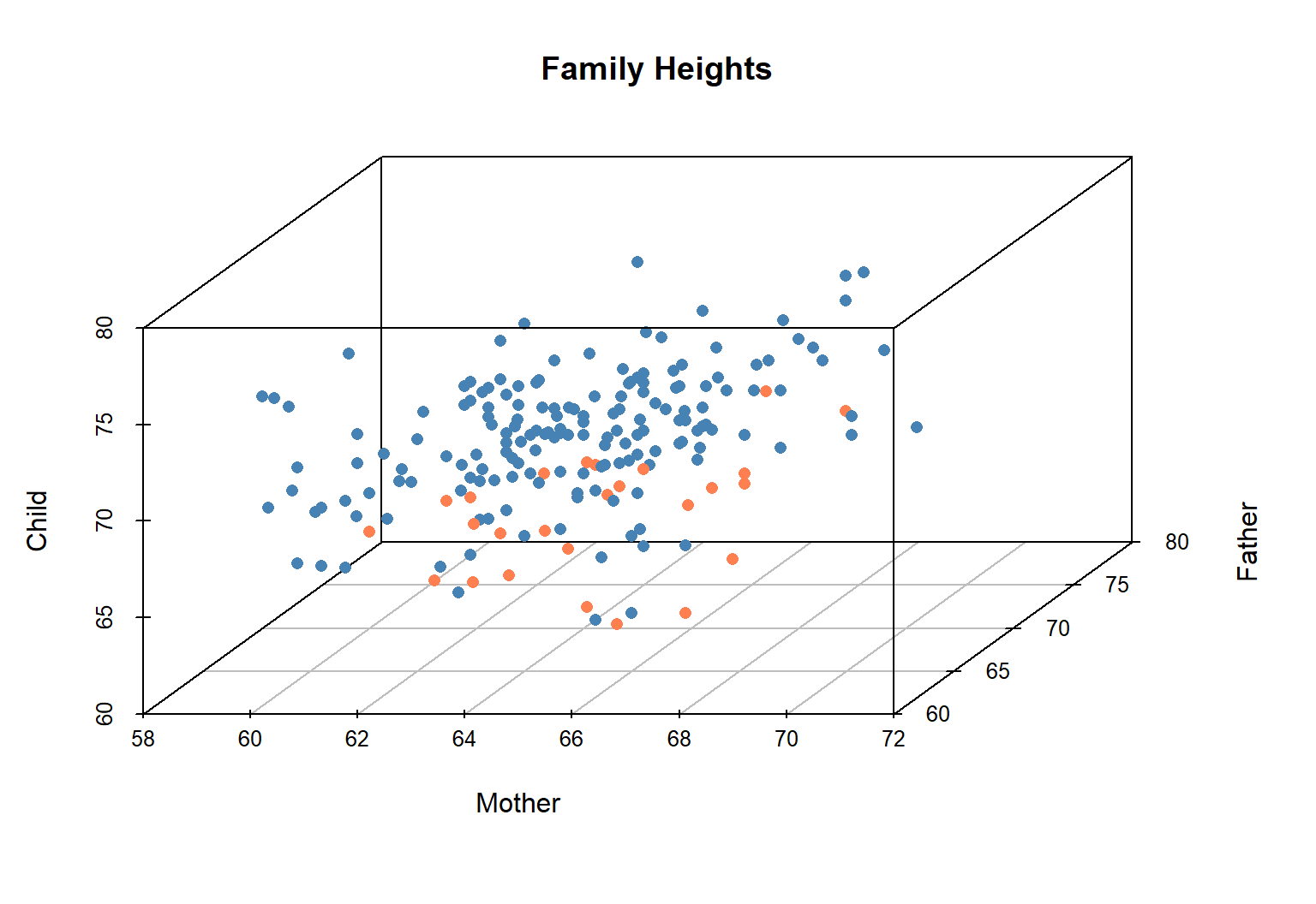
Figure 1: Family heights: sons (blue), daughters (red)
From Line to Plane
In an earlier chapter, we regressed son’s height on father’s height → regression line
Now: regress son’s height on both parents’ heights → regression plane
\[ \hat{s} = \beta_0 + \beta_m \cdot m + \beta_f \cdot f \]
where \(m\) = mother’s height, \(f\) = father’s height
The Regression Plane
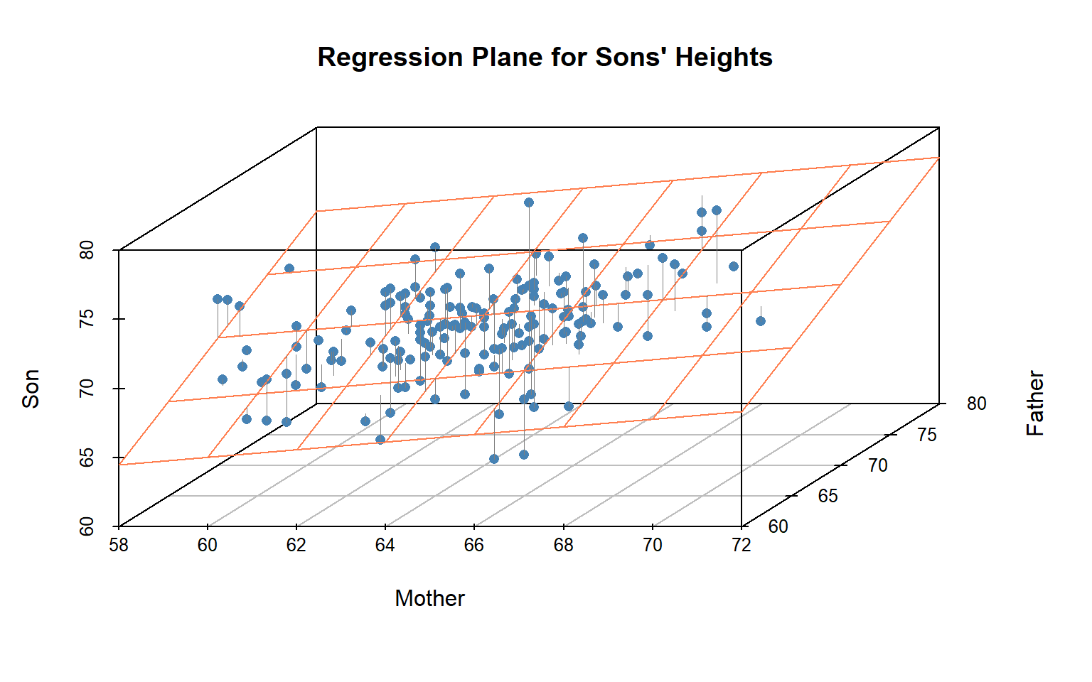
Figure 2: Regression plane with residual segments
Fitted Coefficients
| Term | Coefficient |
|---|---|
| Intercept | 19.94 |
| Mother | 0.28 |
| Father | 0.47 |
Interpretation:
- Each inch of mother’s height → 0.28 inches for son
- Each inch of father’s height → 0.47 inches for son
The Generic Linear Model
Matrix Notation
\[ y_\bullet = X_{\bullet,\bullet} \; \beta_\bullet + \epsilon_\bullet \]
| Symbol | Name | Dimension |
|---|---|---|
| \(y_\bullet\) | Response (target) | \(n \times 1\) |
| \(X_{\bullet,\bullet}\) | Feature matrix | \(n \times d\) |
| \(\beta_\bullet\) | Coefficients | \(d \times 1\) |
| \(\epsilon_\bullet\) | Residuals | \(n \times 1\) |
Feature Space
The columns of \(X\) span a subspace called feature space:
\[ \text{col}(X) = \text{span}(x_{\bullet,1}, \ldots, x_{\bullet,d}) \]
Any prediction \(\hat{y} = X\beta\) is a linear combination of feature vectors:
\[ \hat{y}_\bullet = \beta_1 x_{\bullet,1} + \cdots + \beta_d x_{\bullet,d} \]
So \(\hat{y}\) must lie in \(\text{col}(X)\).
The Central Question
Given \(y_\bullet\) and \(X_{\bullet,\bullet}\):
Find \(\beta_\bullet\) that minimizes \(\|\epsilon_\bullet\|\)
This is the least-squares problem.
Geometric interpretation
Find the point in feature space closest to \(y\).
Geometry of Least Squares
Distance and Norms
The Euclidean norm (length) of vector \(v\):
\[ \|v_\bullet\|_2 = \sqrt{\sum_{\nu=1}^{n} v_\nu^2} \]
Minimizing \(\|\epsilon\|^2\) is the least-squares criterion:
\[ \min_\beta \sum_{\nu=1}^{n} (y_\nu - \hat{y}_\nu)^2 \]
Inner Products
The inner product of vectors \(v\) and \(w\):
\[ \langle v, w \rangle = v^\top w = \sum_{\nu=1}^{n} v_\nu w_\nu \]
Key properties:
- \(\|v\|^2 = \langle v, v \rangle\)
- \(v \perp w\) (orthogonal) when \(\langle v, w \rangle = 0\)
Inner products connect to covariance and correlation.
The Projection Insight
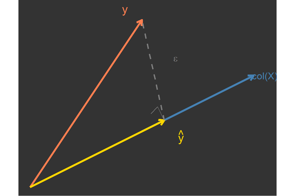
Theorem: The least-squares solution \(\hat{y}\) is the orthogonal projection of \(y\) onto \(\text{col}(X)\).
Why Orthogonal?
The residual \(\epsilon = y - \hat{y}\) is perpendicular to feature space.
Intuition: If \(\epsilon\) had any component along \(\text{col}(X)\), we could reduce its length by adjusting \(\hat{y}\).
Mathematically: \(\epsilon \perp x_{\bullet,j}\) for every feature vector \(j\).
Centering Data
The Intercept Problem
The regression plane \(\hat{s} = \beta_0 + \beta_m m + \beta_f f\) doesn’t pass through the origin.
Problem: It’s not a proper subspace (subspaces must contain the origin).
Solution: Center the data!
Centering Transformation
Replace each value with its deviation from the mean:
\[ \dot{v}_\nu = v_\nu - \bar{v} \]
After centering:
- Mean of each variable is zero
- The regression “plane” passes through the origin
- No intercept term needed
Matrix Form of Centering
\[ \dot{v}_\bullet = C \; v_\bullet \]
where
\[ C = I - \frac{1}{n} \mathbf{1}\mathbf{1}^\top \]
\(C\) is itself a projection matrix—it projects onto the subspace orthogonal to the constant vector.
The Normal Equations
Deriving the Solution
To minimize \(\|\epsilon\|^2 = \|y - X\beta\|^2\):
Take derivative with respect to \(\beta\), set to zero:
\[ X^\top X \; \hat{\beta} = X^\top y \]
These are the normal equations.
The Projection Matrix
Solving for \(\hat{\beta}\):
\[ \hat{\beta} = (X^\top X)^{-1} X^\top y \]
The predicted values:
\[ \hat{y} = X \hat{\beta} = \underbrace{X(X^\top X)^{-1} X^\top}_{P} y \]
Matrix \(P\) is the projection matrix (or “hat matrix”).
Properties of P
The projection matrix \(P = X(X^\top X)^{-1}X^\top\) satisfies:
Idempotent: \(P^2 = P\)
(Projecting twice = projecting once)
Symmetric: \(P^\top = P\)
(Makes it an orthogonal projection)
Complementary: \((I - P)\) projects onto the orthogonal complement
Orthogonality of Residuals
Since \(\hat{y} = Py\) and \(\epsilon = (I-P)y\):
\[ \hat{y}^\top \epsilon = y^\top P^\top (I-P) y = y^\top (P - P^2) y = 0 \]
Key result
Predicted values and residuals are orthogonal.
Row vs Column Views
Two Ways to See Regression
| View | Space | Dimension |
|---|---|---|
| Row | Observations as points in \(\mathbb{R}^d\) | \(d\)-dimensional |
| Column | Features as vectors in \(\mathbb{R}^n\) | \(n\)-dimensional |
Row View: Fitting a Plane
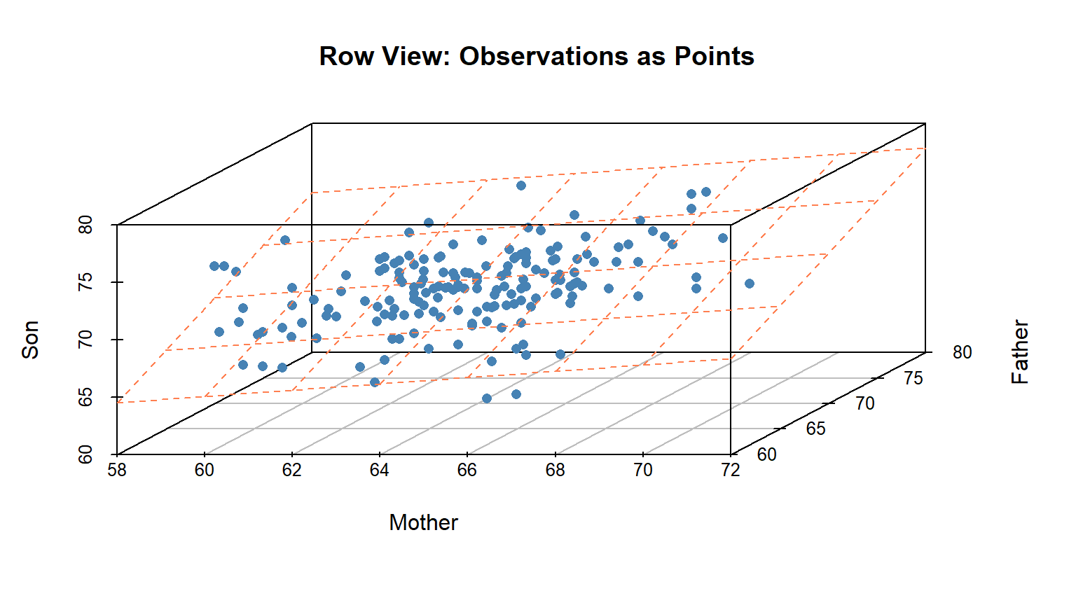
Figure 4: Row view: points in feature space, plane fits through them
Column View: Projection
In \(n\)-dimensional space (one dimension per observation):
- Each feature is a vector of length \(n\)
- \(y\) is a vector of length \(n\)
- \(\hat{y}\) is the projection of \(y\) onto \(\text{span}(x_1, x_2, \ldots, x_d)\)
This is where the linear algebra happens!
Connecting the Views
| Operation | Row View | Column View |
|---|---|---|
| Fit model | Find plane minimizing vertical distances | Project \(y\) onto \(\text{col}(X)\) |
| Residual | Vertical distance to plane | \(y - \hat{y}\) |
| Prediction | Point on plane | Vector in \(\text{col}(X)\) |
Connections to ML
Why This Matters for ML
The projection perspective is foundational for:
Regularization: Ridge regression modifies the projection \[\hat{\beta}_{\text{ridge}} = (X^\top X + \lambda I)^{-1} X^\top y\]
Dimension reduction: PCA finds the “best” low-dimensional subspace
Kernel methods: Project into implicit high-dimensional feature spaces
Neural networks: Each layer performs a linear transformation (projection) followed by a nonlinearity
Covariance as Inner Product
For centered data:
\[ \text{Cov}(x, y) = \frac{1}{n-1} \langle \dot{x}, \dot{y} \rangle \]
Correlation is the cosine of the angle between centered vectors:
\[ r = \frac{\langle \dot{x}, \dot{y} \rangle}{\|\dot{x}\| \; \|\dot{y}\|} \]
This connects regression to the correlation coefficient from Part 1!
Summary
Key Takeaways
Row vs Column: Two complementary views of the same data
Least squares = Projection: \(\hat{y}\) is the orthogonal projection of \(y\) onto feature space
Centering matters: Makes the geometry cleaner (proper subspaces)
P is special: Symmetric, idempotent → orthogonal projection
Residuals ⊥ Features: The defining property of least-squares
Key Formulas
Generic linear model: \[y = X\beta + \epsilon\]
Normal equations: \[X^\top X \hat{\beta} = X^\top y\]
Projection matrix: \[P = X(X^\top X)^{-1}X^\top\]
Predicted values: \[\hat{y} = Py\]
Exercises
Team Exercise 1: By Hand
Let \(y = (3, 1, 2)^\top\) and \(x = (1, 2, 2)^\top\).
- Find the projection \(\hat{y}\) of \(y\) onto \(\text{span}(x)\)
- Compute the residual \(\epsilon = y - \hat{y}\)
- Verify that \(\epsilon \perp x\)
Team Exercise 2: Interpretation
For the Galton height regression:
- What does it mean geometrically that \(\hat{y} \in \text{col}(X)\)?
- Why must the residuals be orthogonal to every column of \(X\)?
- If we added a third predictor (e.g., sibling count), how would the geometry change?
Team Exercise 3: Correlation as Geometry
For centered vectors \(\dot{x}\) and \(\dot{y}\):
- Show that \(r^2 = \cos^2(\theta)\) where \(\theta\) is the angle between them
- What does \(r = 1\) mean geometrically?
- What does \(r = 0\) mean geometrically?
Resources
References
Statistics by Freedman, Pisani, Purves — intuitive treatment of regression
Linear Algebra and Its Applications by Strang — definitive LA text
Introduction to Statistical Learning (ISLR2) — regression in ML context
The Elements of Statistical Learning — advanced treatment