Principal Component Analysis

Finding Directions of Maximum Variance

EDA for Machine Learning

What is PCA?

The Core Question

Given a dataset with multiple features, we ask:

Core Question

Along which directions do the features vary most?

Let’s build intuition through examples before formulas.

Example 1: Galton Heights (2D)

Father and son heights from Galton’s 1885 study:
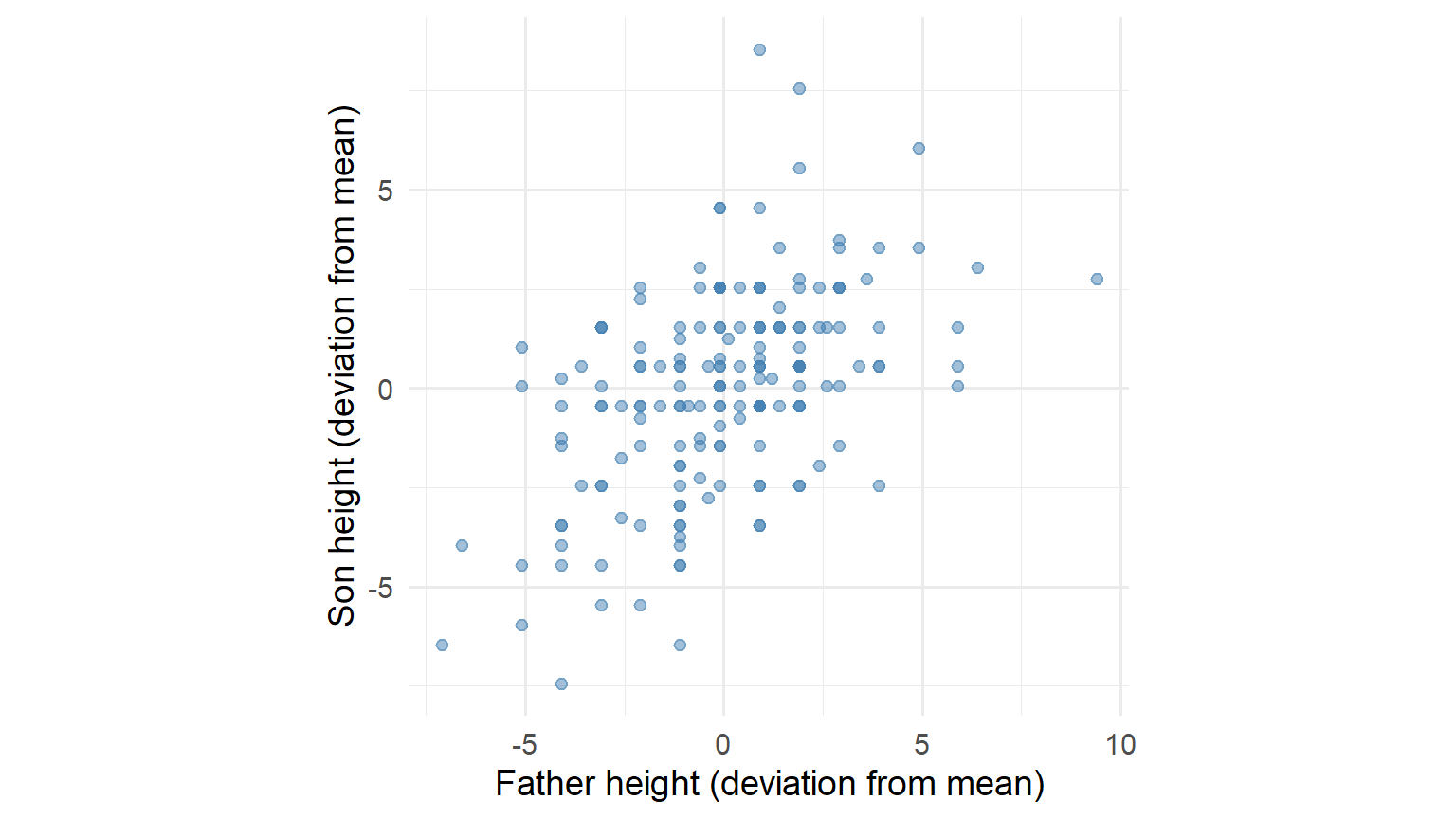
Figure 1: Father-son heights (centred)

The cloud of points has a clear direction of elongation.

Finding PC1: Maximum Variance
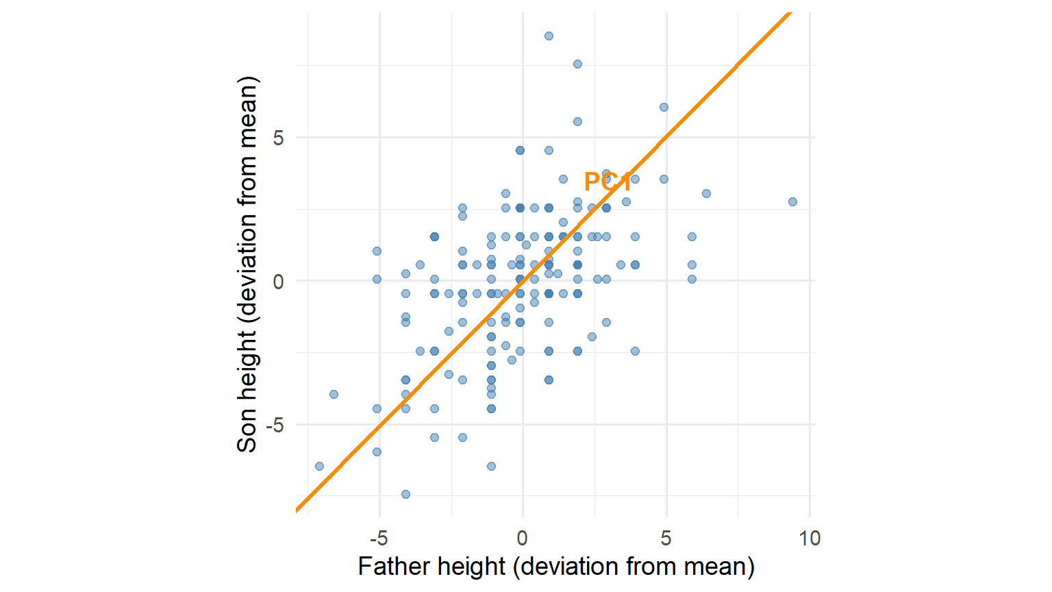
Figure 2: PC1 captures the direction of greatest spread

PC1 is the line that captures the most variance when we project onto it.

PC2: Orthogonal to PC1
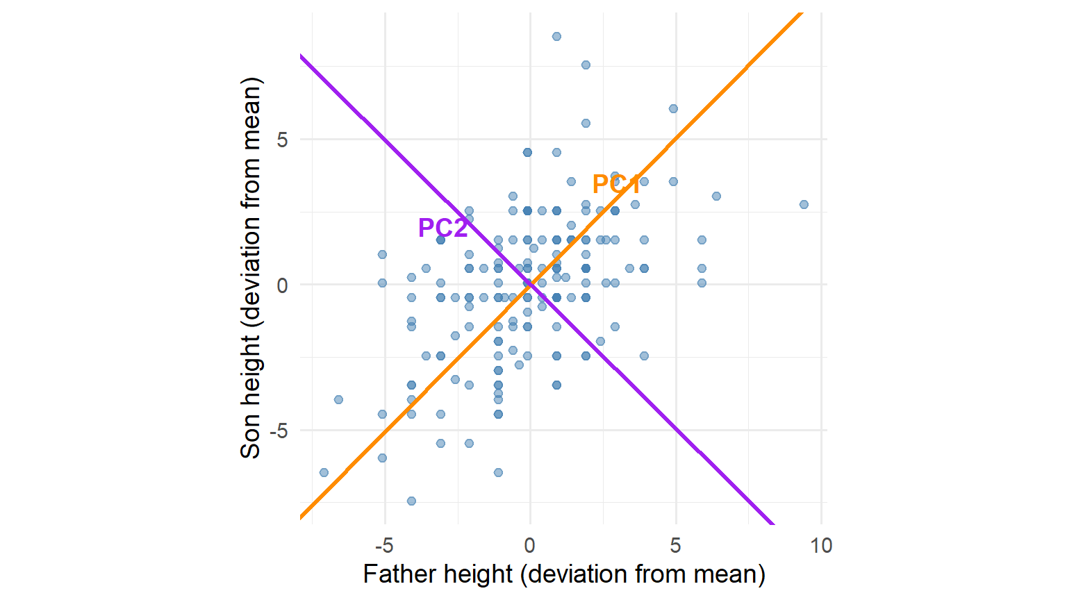
Figure 3: PC1 and PC2 form an orthogonal basis

PC2 captures the remaining variance, orthogonal to PC1.

Galton: Variance Explained

Component Variance Explained
PC1 75.0%
PC2 25.0%

In 2D, PCA simply rotates the coordinate system to align with the data’s natural axes of variation.

Example 2: US Arrests (4D)

From McNeil (1977): violent crime rates per 100,000 population (1973)

Variable Description
Assault Assault arrests
Rape Rape arrests
Murder Murder arrests
UrbanPop Percent urban population

With 4 variables, we can’t simply “look” at the data.

Visualizing 4 Variables

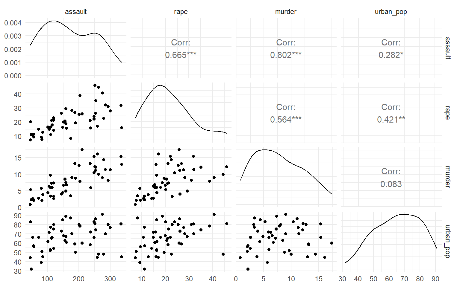
Figure 4: US Arrests: pairwise scatter plots

What Do We See?

Strong correlations among crime variables:

  • Murder–Assault: \(r \approx 0.80\)
  • Murder–Rape: \(r \approx 0.56\)
  • Assault–Rape: \(r \approx 0.67\)

The data don’t fill 4D space—they lie near a lower-dimensional structure.

US Arrests: PCA Results

Component Variance Explained
PC1 62.4%
PC2 24.4%
PC3 9.0%
PC4 4.3%

PC1 alone captures 62% of the variance in four variables.

What Does PC1 Represent?

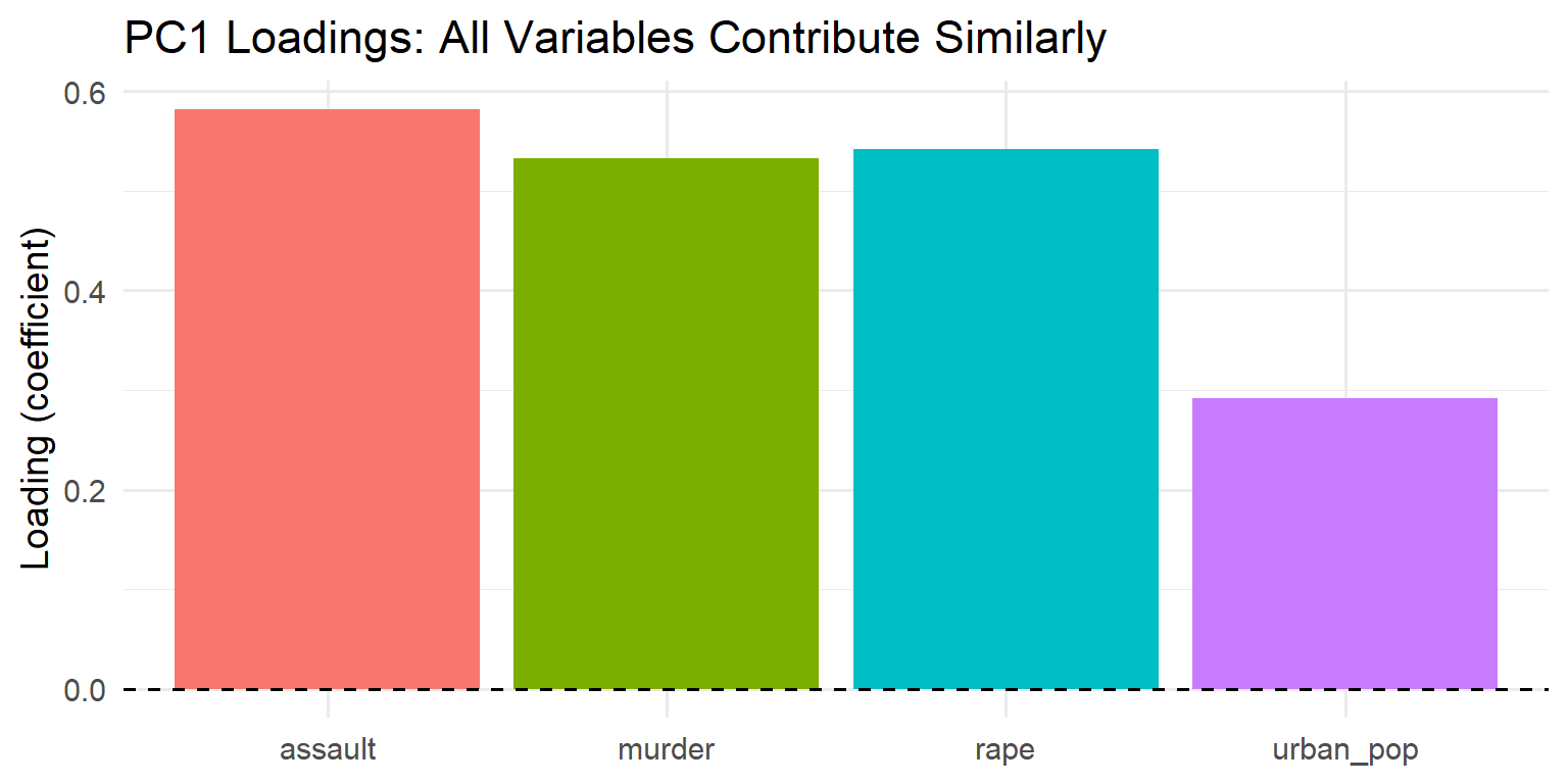
Figure 5: US Arrests: PC1 loadings

All loadings are similar in magnitude—PC1 is a weighted average: a “crime index.”

PC1 Scores: A Crime Index
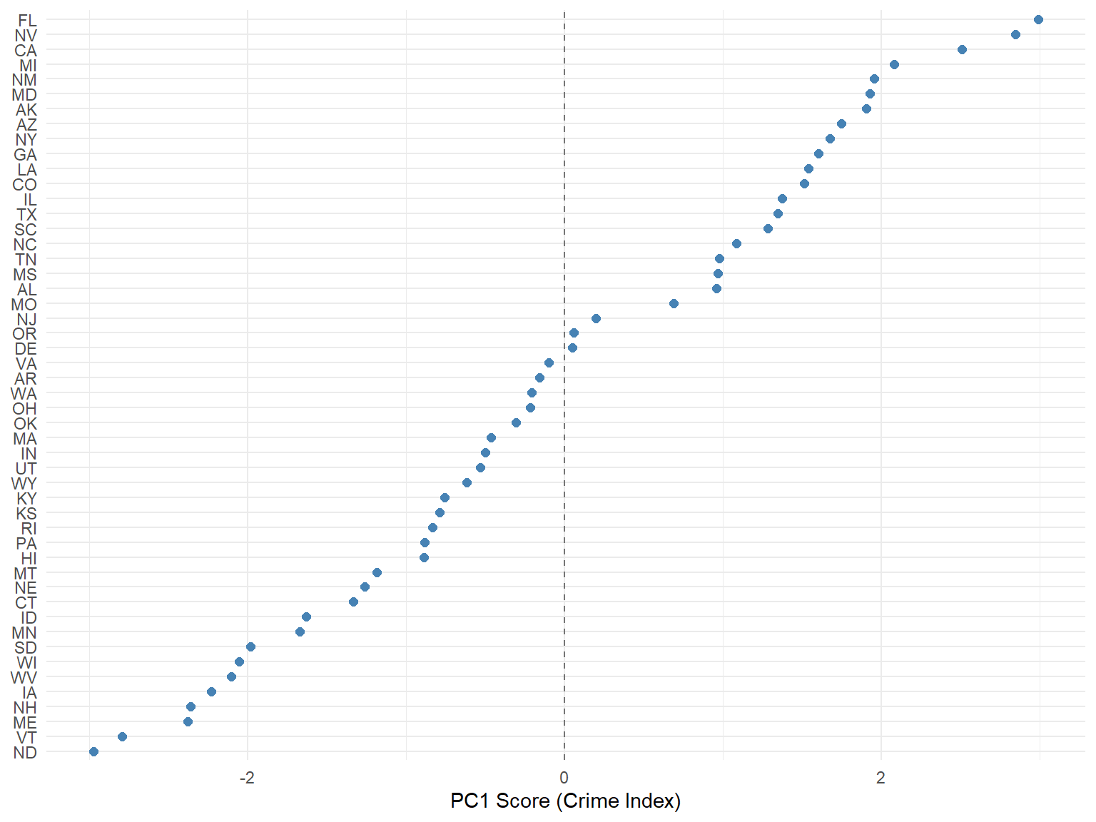
Figure 6: States ranked by PC1 score (crime index)

3D Visualization with PC1

Figure 7: US Arrests in 3D, colored by PC1 score

The gradient shows PC1 capturing the main axis of variation.

Light Explanation: What is PCA Doing?

PCA in One Sentence

PCA finds orthogonal directions that maximize variance, ordered from most to least important.

Mathematically: Find unit vector \(\mathbf{v}_1\) that maximizes \(\text{Var}(\mathbf{X}\mathbf{v}_1)\).

Geometrically: Rotate coordinates to align with the data’s natural axes of spread.

But why would we want to do this?

Why Do We Need PCA?

The Curse of Dimensionality

Modern datasets often have many features:

Domain Typical Features
Genomics 20,000+ genes
Images 1,000,000+ pixels
Text 100,000+ terms
Sensors 1,000s of channels

High dimensions cause problems.

Problem 1: Distances Become Meaningless

In high dimensions, all points become approximately equidistant.
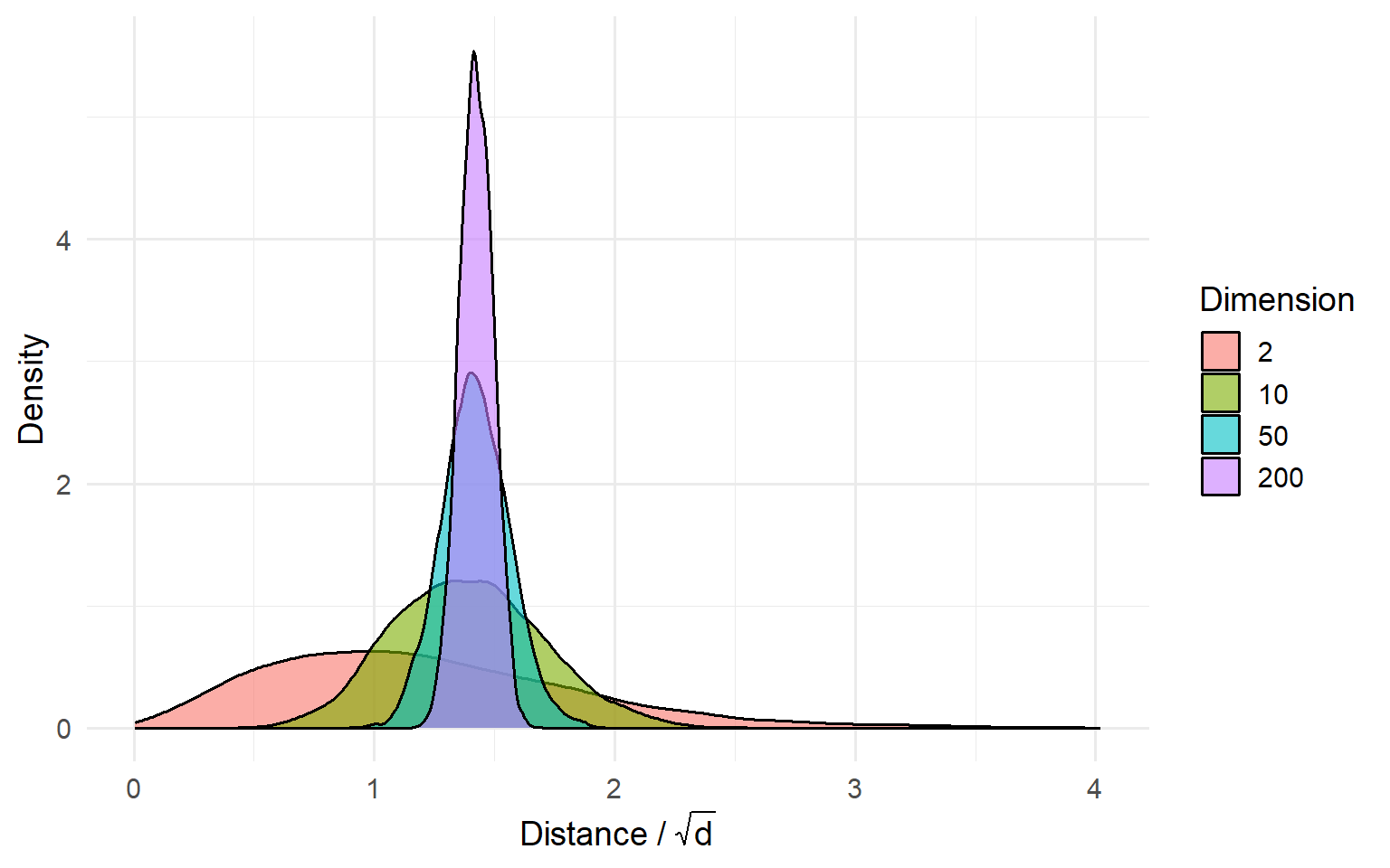
Figure 8: Distribution of pairwise distances as dimension increases

The distributions concentrate—distances lose discriminative power.

Problem 2: Space Becomes Empty
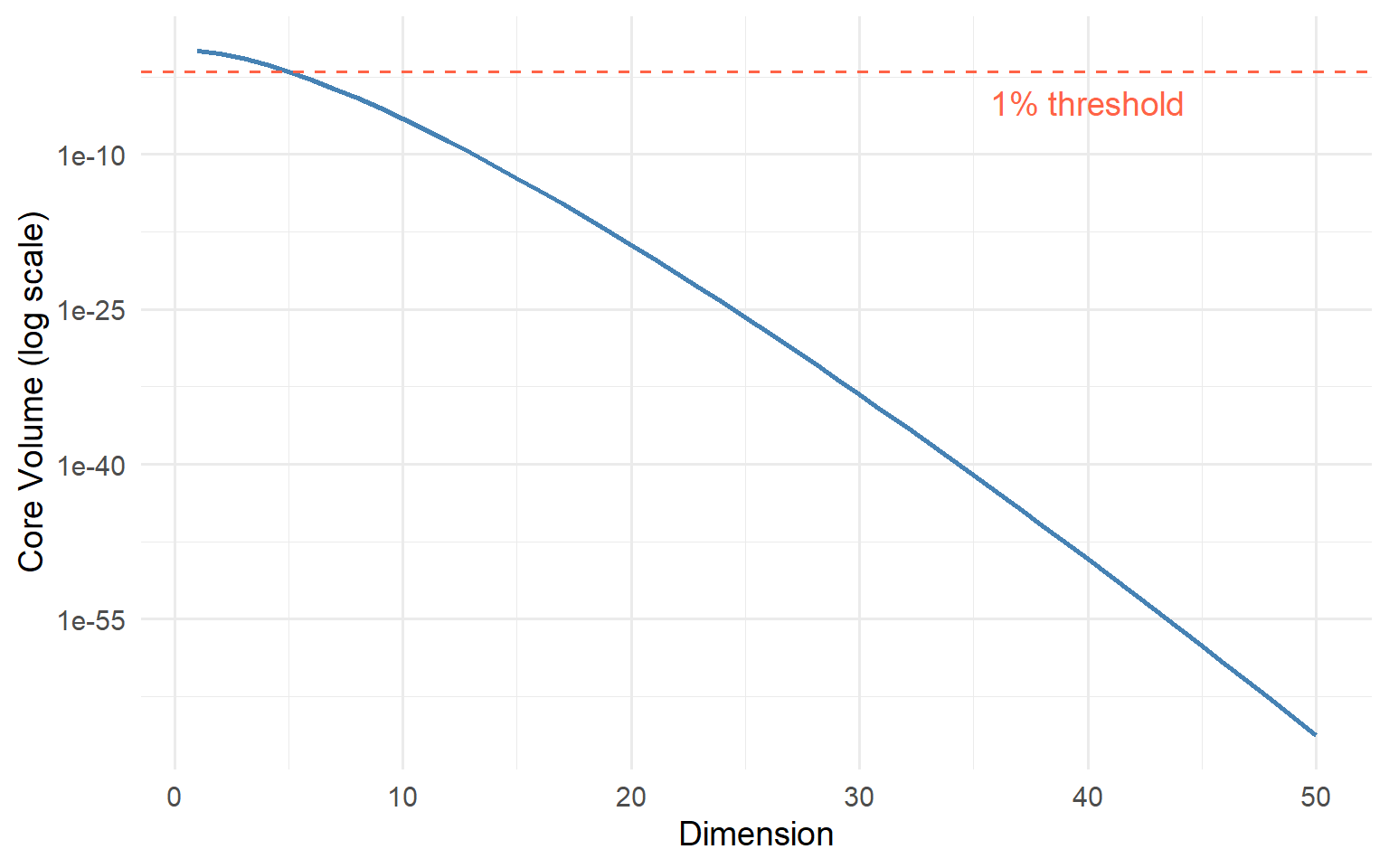
Figure 9: Volume of ball inscribed within unit cube vanishes in high dimensions

In 50 dimensions, 99%+ of the volume is in the “corners.”

Problem 3: Estimation Burden

With \(d\) features, a covariance matrix has \(\frac{d(d+1)}{2}\) parameters.

Features Covariance Parameters
10 55
100 5,050
1,000 500,500
10,000 50,005,000

Without dimension reduction, we need impossibly large samples.

The Opportunity

Donoho (2000)

While randomly generated high-dimensional data behave pathologically, actual data often occupy much lower-dimensional structures.

Examples:

  • Crime rates are correlated (not independent)
  • Chemical properties are constrained by fermentation
  • Gene expression is regulated by pathways

How PCA Addresses the Curse

The PCA Solution

Compress the data to a lower-dimensional subspace that retains most of the variance.

If the first \(k\) principal components capture 90% of the variance:

  • Reduce from \(d\) dimensions to \(k\)
  • Distances become meaningful again
  • Estimation becomes tractable

Full Example: Wine Quality

The Wine Quality Dataset

Statistic Value
Observations 6,497
Features 11
Red wines 1,599
White wines 4,898

11 chemical properties measured on ~6,500 wines.

Question: Can PCA discover the red/white distinction without being told about color?

The Scaling Decision

Table 1
feature max min range
total_so2 440.0 6.0 434.0
free_so2 289.0 1.0 288.0
res_sugar 65.8 0.6 65.2
fix_acidity 15.9 3.8 12.1
alcohol 14.9 8.0 6.9

Variables have very different scales. Without scaling, total sulfur dioxide would dominate.

Wine Quality: PCA

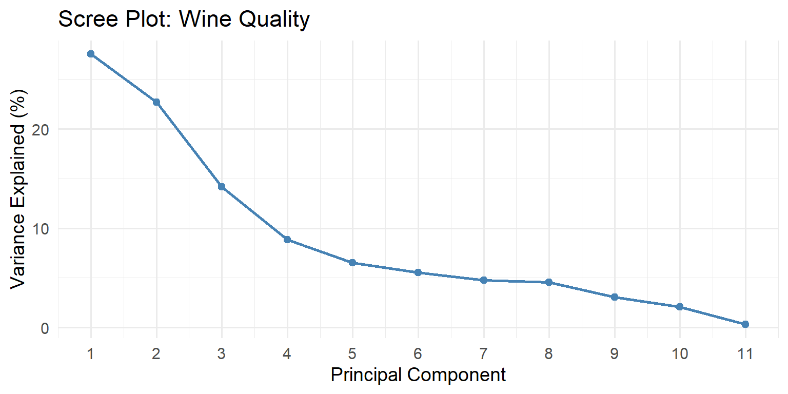
Figure 10: Scree plot: variance explained by each PC

First 4 components capture ~75% of variance.

PC1 vs PC2: The Reveal
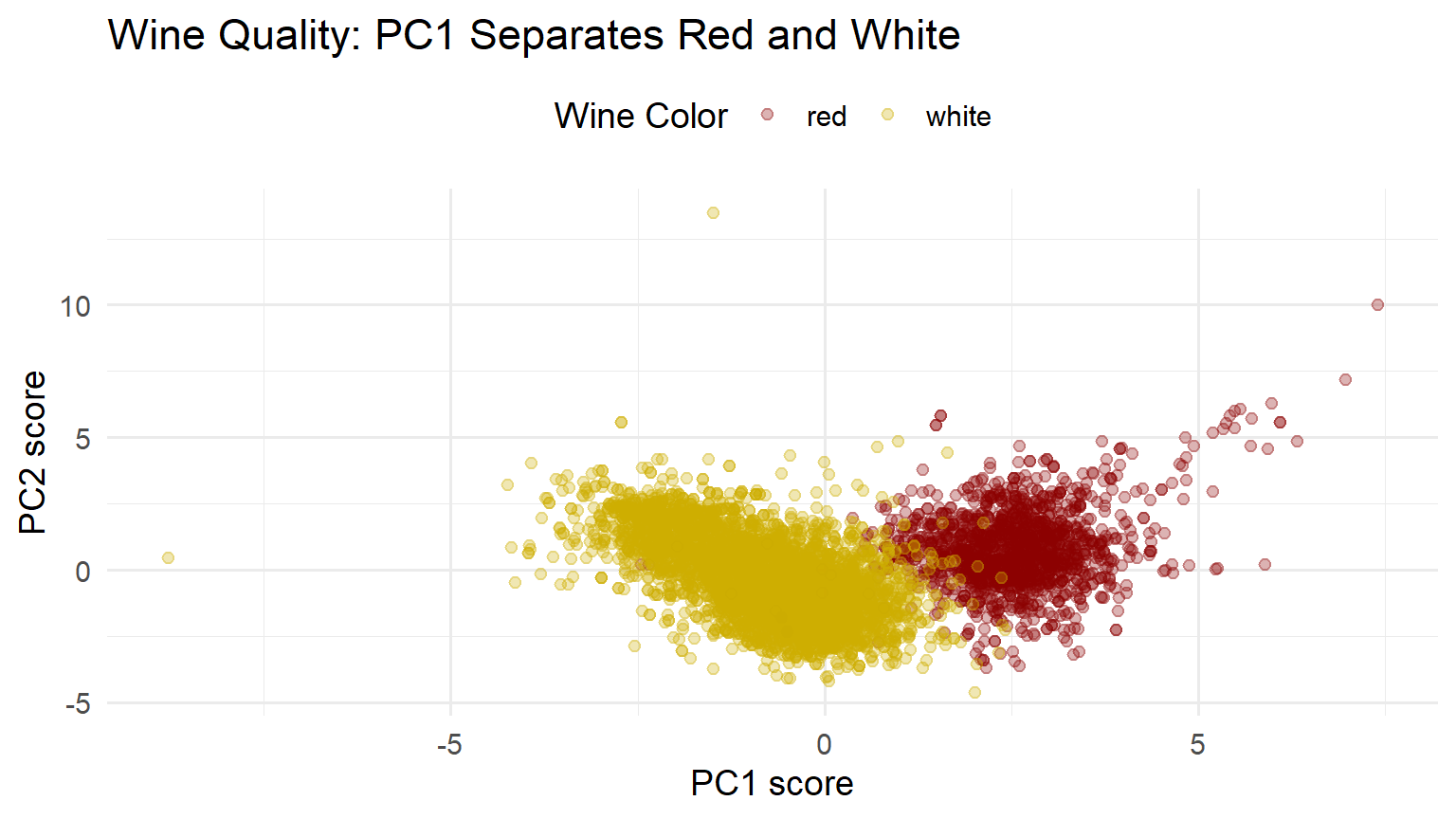
Figure 11: Wine samples projected onto first two principal components

Unsupervised Discovery

Key Insight

PCA separated red and white wines without knowing about color labels.

The chemical properties that vary most across wines happen to distinguish red from white.

This is the power of unsupervised learning: discovering structure the analyst didn’t anticipate.

Interpreting the Loadings

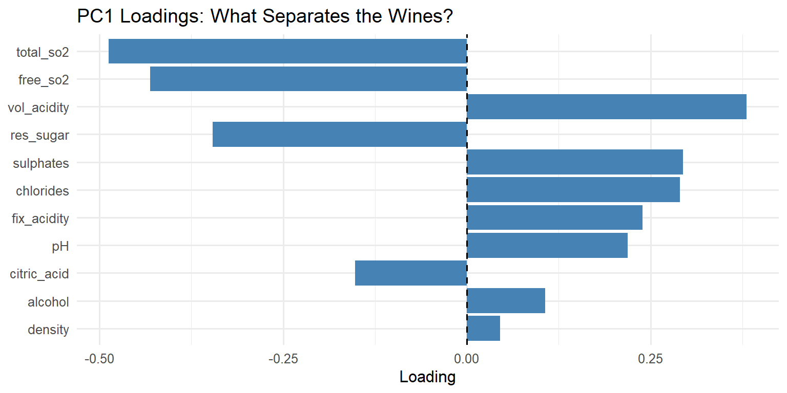
Figure 12: Which variables drive PC1?

PC1: Sulfur compounds (negative) vs volatile acidity/chlorides (positive)

The Algebra of PCA

Notation

Let \(X_{\bullet,\bullet}\) be the centred \(n \times d\) feature matrix.

  • Rows: observations
  • Columns: features (mean = 0)

The covariance matrix:

\[ \text{Cov}(X) = \frac{1}{n-1} X^\top X \]

First Principal Component

The first PC is a linear combination:

\[ c_{\bullet,1} = X_{\bullet,\bullet} \, v_{\bullet,1} \quad \text{with } \|v_{\bullet,1}\| = 1 \]

The vector \(v_{\bullet,1}\) maximizes variance:

\[ \text{var}(c_{\bullet,1}) = \max \left\{ \text{var}(X v) : \|v\| = 1 \right\} \]

The Eigenvalue Solution

Key Result

\(v_{\bullet,1}\) is the eigenvector of \(X^\top X\) with largest eigenvalue \(\sigma_1^2\).

\[ X^\top X \, v_{\bullet,1} = \sigma_1^2 \, v_{\bullet,1} \]

The eigenvalue \(\sigma_1^2\) equals the variance of \(c_{\bullet,1}\) (up to factor \(n-1\)).

Subsequent Components

The \(k\)th principal component maximizes variance subject to orthogonality:

\[ c_{\bullet,k} = X \, v_{\bullet,k} \quad \text{where } v_{\bullet,k} \perp v_{\bullet,1}, \ldots, v_{\bullet,k-1} \]

Solution: \((v_{\bullet,1}, \ldots, v_{\bullet,d})\) are the eigenvectors of \(X^\top X\), ordered by decreasing eigenvalue.

Why PCA Has a Closed Form

Why PCA Is Special

We solve directly via eigenvalue decomposition—no iteration needed.

Contrast with:

  • \(k\)-means: iterates to local optimum
  • Topic models: requires MCMC or variational inference
  • Neural networks: gradient descent

The closed form exists because maximizing a quadratic form (variance) subject to a quadratic constraint (unit norm) yields a linear eigenvalue problem.

Computation: SVD

If \(X = U \Sigma V^\top\), then:

  • Columns of \(V\): Principal component directions (\(v_{\bullet,k}\))
  • Diagonal of \(\Sigma\): Square roots of eigenvalues (\(\sigma_k\))
  • Columns of \(U \Sigma\): Scores (\(c_{\bullet,k}\))

Using prcomp() in R

Code
# Basic PCA workflow
pca_result <- prcomp(X, center = TRUE, scale. = TRUE)

# Loadings (PC directions)
pca_result$rotation

# Scores (observations in PC space)
pca_result$x

# Standard deviations (sqrt of eigenvalues)
pca_result$sdev

Note: scale. = TRUE standardizes features to unit variance—essential when features are on different scales.

Summary

Key Takeaways

  1. PCA finds directions of maximum variance — these capture the most information about differences among observations
  1. Closed-form solution via eigenvalue decomposition — no iteration required
  1. Dimension reduction — project onto first \(k\) PCs to reduce noise and enable visualization
  1. Unsupervised — uses only feature covariance, not labels

Key Formulas

Principal component: \[c_{\bullet,k} = X_{\bullet,\bullet} v_{\bullet,k}\]

Eigenvalue problem: \[X^\top X \, v_{\bullet,k} = \sigma_k^2 \, v_{\bullet,k}\]

Variance explained: \[\text{var}(c_{\bullet,k}) \propto \sigma_k^2\]

Score (projection): \[\text{score}_{i,k} = \langle x_{i,\bullet}, v_{\bullet,k} \rangle\]

Connections to Part 2

Chapter Subspace Basis Determined by
7: Regression \(\text{col}(X)\) Model specification
8: PCA Principal components Data covariance
9: LDA Discriminant directions Class labels

All three use orthogonal projection—they differ in how the target subspace is determined and used.

Looking Ahead

Chapter 9: Linear Discriminant Analysis

  • What if class labels are available?
  • Find directions that separate classes, not just maximize variance
  • Supervised counterpart to PCA

The Contrast

PCA asks: “Where is variance?”

LDA asks: “Where are classes separated?”

Exercises

Team Exercise 1: By Hand

For the \(4 \times 2\) matrix:

\[ X = \begin{pmatrix} 2 & 3 \\ 4 & 5 \\ 6 & 7 \\ 8 & 9 \end{pmatrix} \]

  1. Center the columns
  2. Compute \(X^\top X\) for the centered matrix
  3. Find eigenvalues and eigenvectors
  4. What proportion of variance does PC1 capture?

Team Exercise 2: Scaling

A researcher measures height (cm) and weight (kg) for patients.

  1. Without scaling, which variable will dominate PC1? Why?
  2. The researcher converts height to meters. How does this change PCA?
  3. When should you scale features before PCA?

Team Exercise 3: Interpretation

For the US Arrests data:

  1. All crime variables load positively on PC1. What does a high PC1 score mean?
  2. Murder and Rape have opposite signs on PC2. What does this PC capture?
  3. If you had to create a single “crime index,” would you use PC1? What are the trade-offs?

Team Exercise 4: PCA vs Regression

Both PCA and regression involve projection. Explain:

  1. For each method, how is the subspace determined and used?
  2. Why might maximum-variance directions differ from predictive directions?
  3. Design a 2D example where PC1 is useless for predicting a response.

Resources

References