| Function | Distribution |
|---|---|
| [d,p,q,r]norm | Normal |
| [d,p,q,r]unif | Uniform |
| [d,p,q,r]exp | Exponential |
| [d,p,q,r]gamma | Gamma |
| [d,p,q,r]beta | Beta |
| [d,p,q,r]t | Student t |
| [d,p,q,r]chisq | Chi-squared |
Statistical Simulation
Exploring What-If Scenarios
Chapter 4
Why Simulate?
The Central Question
How might our plans, methods, model \(\ldots\) fail?
Simulation lets us explore scenarios we can’t observe directly.
Generate data from known processes → see how methods behave.
Uses of Simulation
- Compare methods: Which estimator performs better?
- Assess robustness: What happens with outliers? Small samples?
- Understand systems: How does randomness propagate?
- Quantify uncertainty: How precise are our estimates?
The EDA Connection
Simulation extends EDA beyond the data we have.
“What would happen if \(\dots\)?”
- \(\dots\) the sample size were larger?
- \(\dots\) the distribution had heavier tails?
- \(\dots\) there were outliers?
Simulation lets us explore failure modes before they occur in practice.
Random Number Generation
R’s Distribution Functions
For each distribution, R provides four functions:
| Prefix | Function | Example |
|---|---|---|
d |
density/mass | dnorm(0) → 0.399 |
p |
cumulative probability | pnorm(1.96) → 0.975 |
q |
quantile (inverse CDF) | qnorm(0.975) → 1.96 |
r |
random generation | rnorm(10) → 10 values |
Continuous Distributions (selected)
See ?Distributions for a complete list.
Discrete Distributions (selected)
| Function | Distribution |
|---|---|
| [d,p,q,r]binom | Binomial |
| [d,p,q,r]pois | Poisson |
| [d,p,q,r]geom | Geometric |
| [d,p,q,r]nbinom | Negative Binomial |
The Poisson is the “law of rare events”—the limit of Binomial\((n, p)\) as \(n \to \infty\) and \(p \to 0\) with \(np \to \lambda\).
Generating Random Samples
Key insight: We specify the distribution; R generates samples.
Comparing Estimators
Mean vs. Median
Both estimate the center of a symmetric distribution.
Mean: \(\hat{\mu} = \frac{1}{n}\sum_{i=1}^n X_i\)
Median: \(\hat{m}\) = middle value (or average of two middle values)
Which is better? It depends on the distribution.
The Efficiency Question
For normal data, theory tells us:
\[\frac{\text{Var}(\hat{m})}{\text{Var}(\hat{\mu})} \approx \frac{\pi}{2} \approx 1.57\]
The median has 57% higher variance than the mean.
Can we verify this by simulation?
Simulation Design
Simulation Results
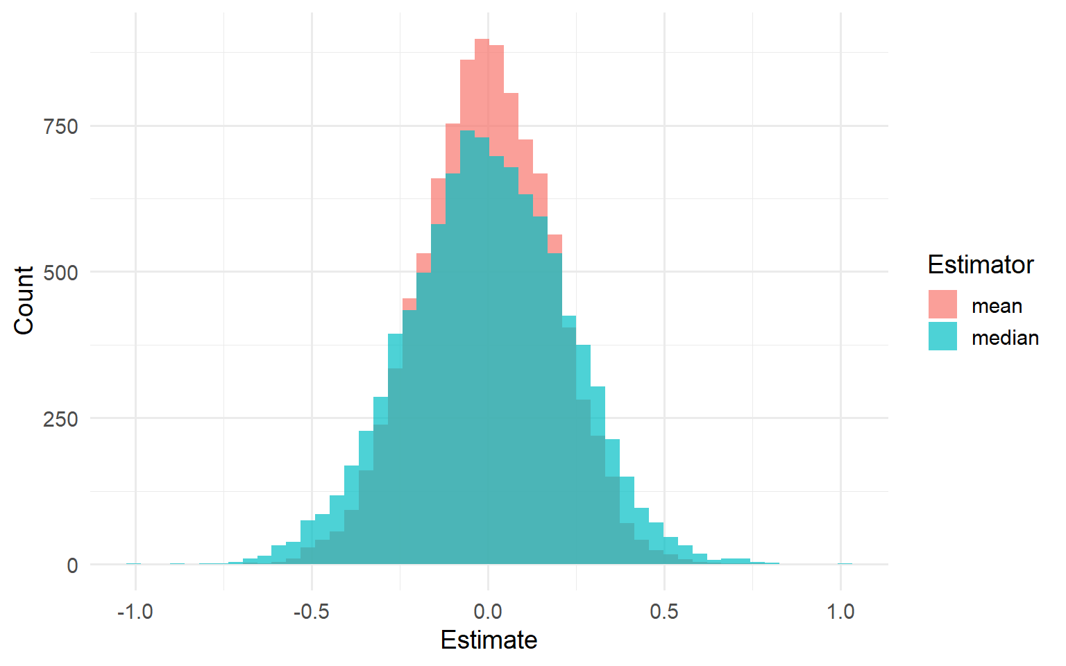
Figure 1: Sampling distributions of mean and median (n=30, R=10,000)
Verifying Theory
| Estimator | Variance | Std Error |
|---|---|---|
| Mean | 0.0338 | 0.1837 |
| Median | 0.0512 | 0.2263 |
Variance ratio: 1.517 (theory: \(\pi/2 \approx\) 1.571)
Simulation confirms the theoretical result.
Why This Matters
We verified a known result. But simulation shines when:
- Theory is intractable
- Assumptions are violated
- We need to compare many methods
EDA application: “How would my estimator behave if the data were slightly different?”
Monte Carlo Methods
Estimating π
Classic example: estimate \(\pi\) by random sampling.
Idea: A quarter circle of radius 1 has area \(\pi/4\).
- Generate random points \((X, Y)\) uniform on \([0,1]^2\)
- Count points inside the quarter circle: \(X^2 + Y^2 < 1\)
- Proportion inside \(\approx \pi/4\)
Visual Intuition
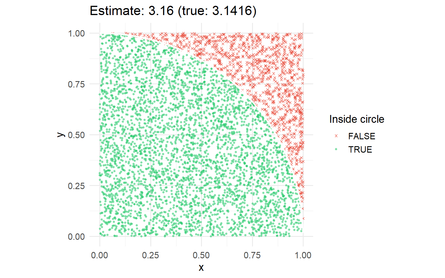
Figure 2: Monte Carlo estimation of π
The Monte Carlo Principle
To estimate \(E[g(X)]\):
\[\hat{\theta} = \frac{1}{n}\sum_{i=1}^n g(X_i)\]
where \(X_1, \ldots, X_n\) are random samples from the distribution of \(X\).
Law of Large Numbers: \(\hat{\theta} \to E[g(X)]\) as \(n \to \infty\)
Convergence Rate
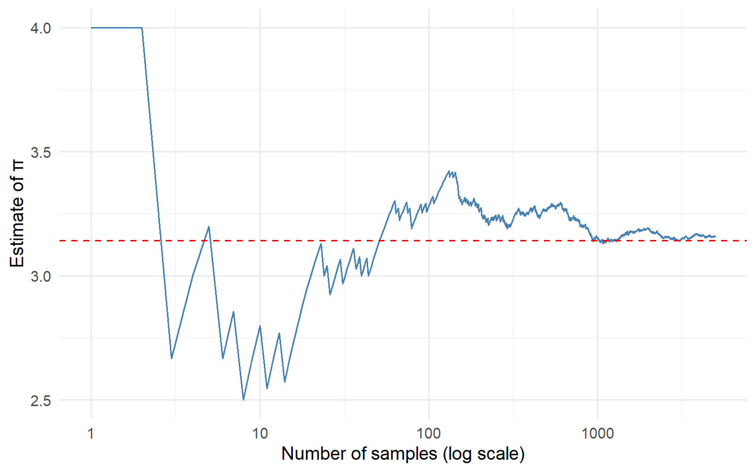
Figure 3: Monte Carlo estimate converges to true value
Standard error decreases as \(1/\sqrt{n}\).
Rare Events
The Problem
What if we want to estimate \(P(Z > 6)\) where \(Z \sim N(0,1)\)?
About 1 in a billion. Naive simulation won’t work.
Naive Approach Fails
[1] 0We’d need billions of samples to see even one event.
Importance Sampling
Key idea: Sample from a different distribution, then reweight.
Instead of sampling from \(p(x)\), sample from \(q(x)\) where rare events are common.
\[E_p[g(X)] = E_q\left[g(X) \cdot \frac{p(X)}{q(X)}\right]\]
The ratio \(w(x) = p(x)/q(x)\) is the importance weight.
Importance Sampling for \(P(Z > 6)\)
Strategy: Shift the normal distribution to center it near 6.
Let \(q(x) = \phi(x - 6)\) (normal centered at 6).
Comparing Estimates
| Method | Estimate |
|---|---|
| True value | 9.87e-10 |
| Importance sampling | 9.92e-10 |
| Naive (n = 10^6) | 0 |
Importance sampling makes the impossible feasible.
Bootstrap
Quantifying Uncertainty
How precise is our estimate?
Classical approach: derive standard error formula.
Bootstrap approach: Resample from the data itself.
The Bootstrap Idea
- Treat the sample as a proxy for the population
- Draw with replacement from the sample
- Compute statistic on each resample
- Use variability across resamples to estimate uncertainty
Bootstrap in Action
Bootstrap Example
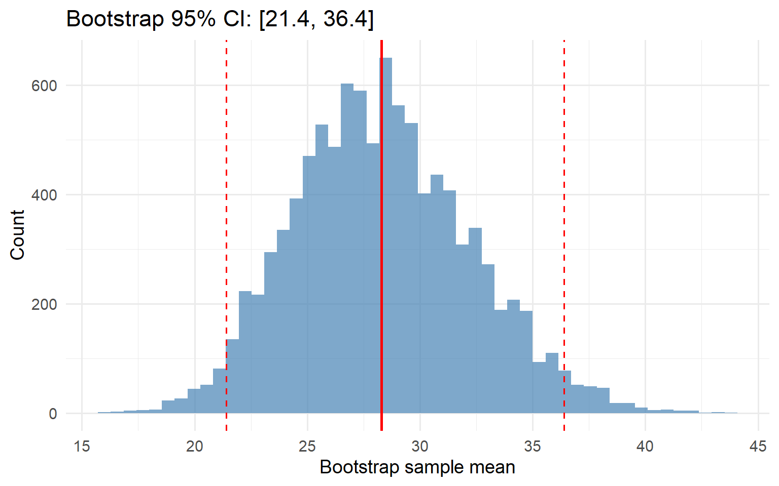
Figure 4: Bootstrap distribution of the sample mean
Normal theory 95% CI: [18.9, 37.7] — similar result.
Bootstrap for Any Statistic
The bootstrap works for almost any statistic:
- Correlation coefficients
- Regression coefficients
- Median, trimmed mean
- Ratios, differences
EDA application: “How much would this pattern change with different data?”
Connections to ML
Simulation in the ML Pipeline
Simulation connects to machine learning:
Cross-validation: Repeatedly resample to estimate generalization error.
Stochastic gradient descent: Random sampling of training batches.
Bayesian ML: MCMC and variational inference sample from posteriors.
Simulation as Model Checking
After fitting a model:
- Simulate data from the fitted model
- Compare simulated data to real data
- Discrepancies reveal model failures
This is the posterior predictive check—simulation for model criticism.
Summary
Chapter 4: Key Takeaways
Simulation explores what-if scenarios before they occur
R provides d/p/q/r functions for common distributions
Monte Carlo methods estimate quantities via random sampling
Importance sampling handles rare events
Bootstrap quantifies uncertainty without formulas
Key Formulas
| Concept | Formula |
|---|---|
| Monte Carlo estimate | \(\hat{\theta} = \frac{1}{n}\sum_{i=1}^n g(X_i)\) |
| Importance weight | \(w(x) = p(x) / q(x)\) |
| Variance ratio (mean vs. median) | \(\pi/2 \approx 1.57\) |
The Simulation Workflow
- Specify the data-generating process
- Generate random samples
- Compute statistics of interest
- Repeat many times
- Summarize the distribution of results
Exercises
Team Exercise 1: Mean vs. Median Efficiency
Verify the variance ratio for normal data:
- Set \(n = 30\) and \(R = 5000\) replications.
- For each replication, generate a sample from
rnorm(), compute mean and median. - Calculate
var(medians) / var(means). Compare to \(\pi/2 \approx 1.57\). - What does this ratio tell us about the relative efficiency of the median?
Team Exercise 2: Heavy Tails and the Cauchy
Repeat Exercise 1, but use rcauchy() instead of rnorm().
- Calculate the sample variance of your \(R\) means. What do you observe?
- Construct a histogram of sample means. Does it look normal?
- What does this imply about the Central Limit Theorem?
Team Exercise 3: Bootstrap Confidence Interval
Use the bootstrap to estimate a 95% CI for the median of mtcars$mpg:
- Resample with replacement \(B = 2000\) times.
- Compute the median for each bootstrap sample.
- Use the 2.5th and 97.5th percentiles as your CI.
- How does the width compare to a bootstrap CI for the mean?
Team Exercise 4: Importance Sampling
Estimate \(P(Z > 4)\) using importance sampling. Compare to pnorm(4, lower.tail = FALSE).
Discussion Questions
When is simulation more trustworthy than mathematical derivation?
A colleague sets
set.seed(42)and runs one simulation. Is this reproducible research?How many bootstrap replications are “enough”?
Resources
- Advanced Statistical Computing by Roger Peng
- Monte Carlo method - Wikipedia
- Bootstrap Methods
- R documentation:
?Distributions