Sampling and Study Design

Why how you collect data matters more than how much

EDA for Machine Learning

Chapter 5

• Opening
• Observational Studies
• Experimental Studies
• Measurement and Uncertainty
• The Role of EDA
• Synthesis
• Exercises
• Appendix: Instructor Notes

Opening

The Big Data Paradox

If we have millions of records, why does sampling theory matter?

Answer: As soon as you ask “what would happen if…” you’re generalizing beyond your data.

ML Connection

Training data should be a sample from the deployment environment.

This is the key insight for a data science audience. Even “big data” is a sample from some larger process. The question is whether it’s a representative sample.

Chapter Roadmap

1. Observational studies: Learning from data you didn’t generate
2. Experimental studies: Learning from conditions you control
   
3. Measurement: Bias, chance error, and uncertainty
4. The role of EDA: Bridging design and modeling

Instructor note: This chapter draws heavily from Freedman, Pisani, and Purves (FPP). The examples are classic but the lessons are timeless.

Observational Studies

Literary Digest, 1936: The Largest Poll in History

Source	FDR Predicted %
Digest	43
Gallup re Digest	44
Gallup re election	56
election result	62

The Digest’s error of 19 percentage points is the largest in polling history.

Pause here to let the numbers sink in. 2.4 million respondents got it catastrophically wrong. 50,000 got it roughly right. This sets up the key lesson.

What Went Wrong?

The Digest sampled from:

• Automobile registrations
• Telephone directories
• Magazine subscription lists

In 1936, these skewed wealthy—and wealthy voters favored Landon.

Selection Bias

The sampling frame excluded the population of interest.

ML Connection

If your training data excludes a subpopulation, your model won’t serve them.

Truman vs. Dewey, 1948:

Quota Sampling Fails

source	Truman	Dewey	Thurmond	Wallace
Crossley	45	50	2	3
Gallup	44	50	2	4
Roper	38	53	5	4
election result	50	45	3	2

All three major polls predicted Dewey by 5+ points. All three were wrong.

This is the famous “Dewey Defeats Truman” headline moment. Ask the class if they’ve seen the photo of Truman holding that newspaper.

Quota Sampling: The Problem

Quota sampling: Match sample demographics to population demographics.

• Interviewers given quotas: X women, Y employed, Z from each region…
• Otherwise free to choose subjects

The hidden bias: Interviewers chose “convenient” subjects within quotas—who tended to vote Republican.

The key insight is that there are many factors influencing voting, and you can’t control for all of them with quotas. Interviewers unconsciously selected people who were easier to interview.

Probability Sampling

Key insight: Too many known and unknown factors to control them all.

Solution: Let chance create a representative sample.

Simple random sampling: Every individual has a known, equal probability of selection.

Hallmark of Probability Sampling

The probability of including any given individual can be calculated in advance.

Practical Probability Sampling

Simple random sampling is often impractical (cost, logistics).

Multi-stage cluster sampling: Randomly select regions → towns → precincts → households

Key features preserved:

• No interviewer discretion in subject selection
• Prescribed procedure involving planned use of chance

Post-1948: Probability Sampling Works

Year	Sample Size	Winner	Gallup %	Actual %	Error
1952	5385	Eisenhower	51	55.1	-4.1
1960	8015	Kennedy	51	49.7	1.3
1976	3439	Carter	48	50.1	-2.1
1984	3456	Reagan	59	58.8	0.2
2000	3571	Bush	48	47.9	0.1
2004	2014	Bush	49	50.6	-1.6

Errors mostly within ±3 percentage points—with samples of 2,000-8,000, not millions.

This is a subset of the full table in the textbook. The point is the contrast with the Literary Digest: smaller samples with probability sampling beat huge samples with biased sampling.

UC Berkeley Admissions: Simpson’s Paradox

In the 1970s, concern arose that graduate admissions were biased against women.

Overall admission rate: Men 44%, Women 35%

But department-by-department analysis told a different story…

This is one of the most famous examples of Simpson’s Paradox. Build the suspense before revealing the twist.

The Paradox Revealed

Most departments admitted a higher percentage of female applicants.

What happened? Women applied disproportionately to departments with lower overall admission rates.

Aggregating across departments reversed the apparent pattern.

ML Connection

A feature (gender) appeared predictive of the outcome (admission) only because both were associated with a confounder (department choice). Stratify by potential confounders.

UC Berkeley: The Sampling Lesson

• Data included all applicants in 1973 (not a sample)
• Standard statistical formulas assume probability sampling
• If data aren’t from a probability sample, standard errors don’t apply

ML Connection

Your test set is a sample; your deployment data may not be from the same distribution.

This is a subtle but important point. Many ML practitioners compute confidence intervals on test metrics, but if the test set isn’t representative of deployment, those intervals are meaningless.

Experimental Studies

Why Experiment?

Observational data: Subjects choose their own “treatment”

Confounding: Factors that affect both treatment choice and outcome

Experiment: Researcher assigns treatment, breaking confounding

Draw a simple DAG on the board if you have time: Confounder → Treatment → Outcome, with Confounder also → Outcome. Randomization breaks the Confounder → Treatment arrow.

Salk Vaccine Trial: NFIP Design

Grade	Group	Size	Polio Rate (per 100k)
2	treatment	225000	25
1, 3	control	725000	54
2	no_consent	125000	44

Problems:

• Grade might affect polio transmission
• Consent might be confounded with risk factors

Salk Vaccine Trial: Double-Blind Design

Group	Size	Polio Rate (per 100k)
treatment	200000	28
control	200000	71
no_consent	350000	46

Key insight: Non-consent group had lower rate than placebo group.

Consent itself was confounded with risk!

Higher SES parents were more likely to consent, but their children were at higher risk (less early exposure → less natural immunity). This is a beautiful example of confounding that only became visible with proper randomization.

Double-Blind Design: Why It Matters

Randomization: Consenting parents’ children assigned to vaccine or placebo by chance

Blinding: Neither parents, doctors, nor evaluators knew assignment

This eliminates:

• Selection bias in treatment assignment
• Unconscious bias in outcome measurement

ML Connection

In supervised ML, annotators should not have access to information that could bias their labels. The NFIP’s initial design mirrors label leakage.

The Portacaval Shunt: Design Determines Conclusions

Study Design	Marked Enthusiasm	Moderate	None
no controls	24	7	1
controls not randomized	10	3	2
randomized controlled	0	1	3

The same surgery looked beneficial or useless depending on study design.

This is one of the most striking tables in all of statistics. 75% of uncontrolled studies were enthusiastic; 0% of randomized studies were. The surgery doesn’t work, but bad study design made it look like it did.

The Mechanism of Bias

Design	Surgery Survival %	Control Survival %
randomized	60	60
not randomized	60	45

Surgery patients: ~60% survival in both study types

Control patients: 60% (randomized) vs 45% (non-randomized)

Non-randomized studies used sicker patients as controls.

ML Connection

Evaluating a model on a non-exchangeable test set overstates performance. Randomized train/test splits guard against this bias.

Experimental Design Principles

1. Randomization: Breaks confounding
2. Control group: Provides counterfactual
   
3. Blinding: Prevents unconscious bias in measurement

ML Connection

A/B tests are randomized controlled experiments. Observational “causal” claims require strong assumptions.

Measurement and Uncertainty

NB10: Precision Measurement

NB10: A standard weight, nominally 10 grams

Study: 100 measurements under identical conditions at the National Bureau of Standards

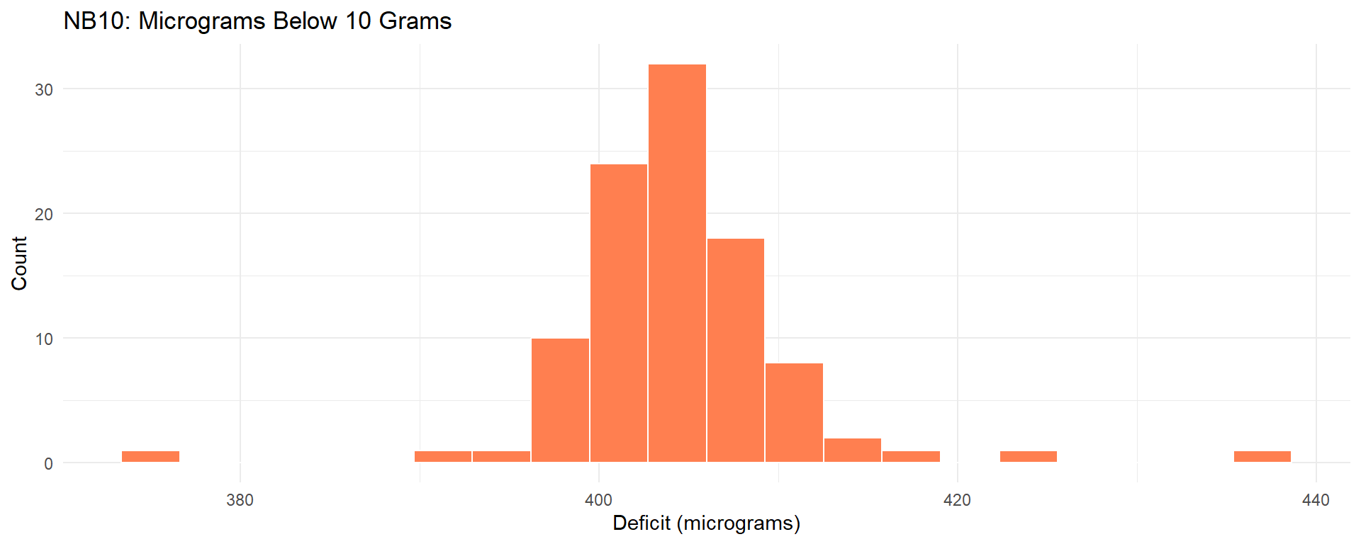
Figure 1

Bias vs. Chance Error

Each measurement = true value + bias + chance error

• Chance error: Varies randomly, averages toward zero
• Bias: Systematic, does not average out

NB10 is biased: It weighs ~405 μg less than 10g

ML Connection

Model error = bias + variance. EDA reveals both.

How Accurate is the Sample Average?

\[\text{SE of mean} = \frac{\text{SD}}{\sqrt{n}}\]

For NB10:

\[\text{SE} = \frac{6.5}{\sqrt{100}} = 0.65 \text{ micrograms}\]

Our estimate of 405 μg is probably within ~2 μg of the true value.

Key Insight

Uncertainty shrinks with \(\sqrt{n}\), not \(n\). Precision and accuracy are distinct.

Outliers and Non-Normality

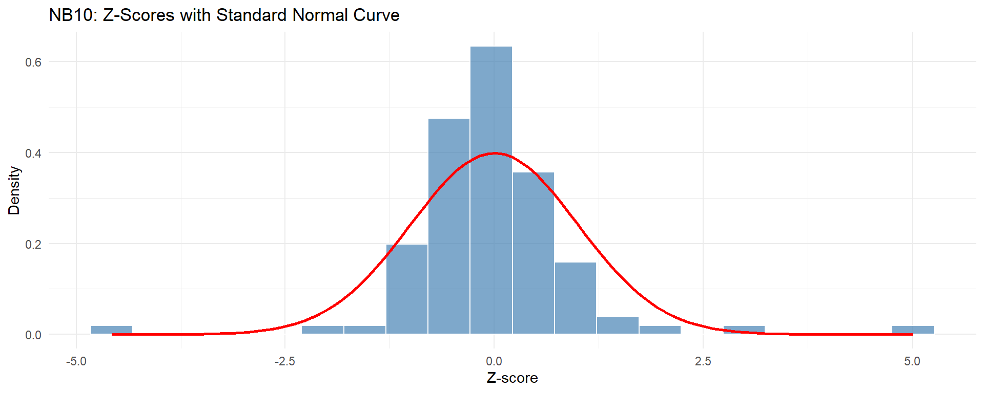
Figure 2

Measurements at z ≈ ±5 would be < 1 in a million under normality.

Even careful measurement processes produce non-normal tails.

ML Connection

Don’t assume normality. Look at your data.

The Role of EDA

EDA Bridges Design and Modeling

Study design determines what data could be collected.

EDA reveals what was actually collected.

EDA answers:

• Does the feature distribution match deployment expectations?
• Are there systematic patterns in missing data?
• Do labels exhibit expected reliability?
• Are there outliers warranting investigation?

This is the bridge to the rest of the course. Study design sets intentions; EDA verifies whether those intentions were achieved.

The Bottom Line

No algorithm can overcome fundamentally flawed data collection.

EDA is the diagnostic step that reveals whether data support the intended use.

The examples in this chapter—from the Literary Digest poll to the NB10 measurements—show that study design flaws are often invisible until the data are examined.

Synthesis

Key Takeaways

1. How data are collected determines what conclusions are valid

2. Sample size without representative sampling is worthless

3. Observational data cannot establish causation without strong assumptions

4. Randomized experiments are the gold standard for causal claims

5. All estimates have uncertainty—quantify it

Key Concepts

Concept	Definition
Selection bias	Sample systematically differs from population
Confounding	Third variable creates spurious association
Randomization	Assignment by chance mechanism
Double-blind	Neither subject nor evaluator knows assignment
Standard error	SD of a sample statistic: \(\sigma / \sqrt{n}\)

Looking Ahead: ML Implications

• Train/validation/test splits are sampling problems

• Distribution shift: Deployment ≠ training distribution

• Fairness: If subgroups are undersampled, models underperform for them

• Causal inference: When can observational data support cause-and-effect claims?

These are the bridges to later ML material. Each of these could be a full lecture in its own right.

Exercises

Team Exercise 1: Observational Studies at Work

Break into teams:

1. Identify 2–3 examples of observational studies in your work context.
2. Which would be most valuable? What questions would they answer?
3. What are the potential pitfalls (confounding, selection bias, etc.)?
4. Could any be converted to experiments? At what cost?

Team Exercise 2: The Quiz Puzzle

A TA gives a 10-question quiz. After grading:

• Average number right: 6.4, SD: 2.0
• Average number wrong: [?], SD: [?]

Fill in the blanks—or do you need the raw data? Explain briefly.

Team Exercise 3: Left-Handedness Puzzle

In a large health survey, the percentage of left-handed respondents decreased from 10% at age 20 to 4% at age 70.

“The data show that many people change from left-handed to right-handed as they get older.”

1. True or false? Explain.
2. If false, what explains the pattern?
3. What study design would test your alternative hypothesis?

Team Exercise 4: Normal Distribution

The 25th percentile of height is 62.2 inches; the 75th is 65.8 inches. If the distribution is normal, find the 90th percentile.

Exercise 1 grounds concepts in participants’ experience. Exercises 2–3 are from FPP and test reasoning about study design. Exercise 4 refreshes familiarity with the normal (Gaussian) distribution.

Discussion Questions

1. What modern datasets might have Literary Digest-style selection bias?

2. When is a randomized experiment unethical or impractical?

3. How would you detect distribution shift between training and deployment?

These are the FPP exercises from the chapter. They reinforce the core concepts and can be used as in-class activities or homework.

Appendix: Instructor Notes

Timing Guide

Section	Slides	Suggested Time
Opening	1-2	5 min
Observational Studies	3-12	25 min
Experimental Studies	13-20	20 min
Measurement/Uncertainty	21-24	15 min
Role of EDA	25-26	5 min
Synthesis	27-32	15 min

Total: ~85 minutes with discussion

Customization Options

For shorter sessions (50 min): Cut slides 8, 12, 24; condense synthesis

For longer sessions: Expand Simpson’s Paradox with actual department data; add more discussion time

For ML-focused audience: Expand “ML Connection” callouts with code examples

For statistics-focused audience: Show the mathematical derivations from FPP

Data Sources

All FPP datasets are loaded from the eda4mldata package:

• lit_digest — Literary Digest 1936 poll
• truman_dewey — 1948 election predictions
• us_elections — Gallup accuracy 1952-2004
• salk_nfip — Salk vaccine NFIP design
• salk_blind — Salk vaccine double-blind design
• portacaval_studies — Portacaval shunt study results
• portacaval_survival — Shunt survival rates
• nb10 — NB10 weight measurements