| book | n_paragraphs | n_words |
|---|---|---|
| Animal Farm | 5 | 553 |
| Butter Battle Book | 4 | 172 |
Topic Models
Discovering Latent Themes
EDA for Machine Learning
Generative Model Recap
From Chapter 10
We established:
- Text → tokens → term-document matrix
- TF-IDF surfaces distinctive words
- Topic models discover latent themes
Now we go deeper: How do topic models work?
The Core Insight
A topic model makes two key assumptions:
- Each document is a mixture of topics
- “This article is 70% business, 30% politics”
- Each topic is a mixture of words
- Business topic: “market”, “profit”, “growth” have high probability
- Politics topic: “congress”, “vote”, “campaign” have high probability
The Generative Story
Imagine generating a document:
Step 1: Choose a mixture of topics for this document
- Topic mixture: “70% Topic A, 30% Topic B”
Step 2: For each word position:
- Roll the topic dice → generate a topic
- From that topic’s word distribution → generate a word
LDA inverts this process: Given documents, infer the topics.
Toy Example: Two Books
The Experiment
Can LDA distinguish two very different books?
Animal Farm (George Orwell, 1945)
- Farm animals overthrow humans, pigs become tyrants
- Allegory for Soviet communism
The Butter Battle Book (Dr. Seuss, 1984)
- Yooks vs Zooks over which side to butter bread
- Allegory for Cold War nuclear arms race
We use Wikipedia’s plot summaries, treating each paragraph as a “document.”
Loading the Texts
Our mini-corpus of paragraphs within plot summaries:
Building the Document-Term Matrix
Code
# Count words per paragraph (our "documents")
af_bbb_counts <- af_bbb_token_tbl |>
  dplyr::mutate(doc_id = paste(src, pdx, sep = "_")) |>
  dplyr::count(doc_id, word)

# Convert to document-term matrix
af_bbb_dtm <- af_bbb_counts |>
  tidytext::cast_dtm(document = doc_id, term = word, value = n)

af_bbb_dtm
<<DocumentTermMatrix (documents: 9, terms: 486)>>
Non-/sparse entries: 598/3776
Sparsity : 86%
Maximal term length: 18
Weighting : term frequency (tf)Fitting LDA with K = 2
We asked for 2 topics—matching our 2 source books.
Can LDA recover the distinction?
Word Distribution \((\beta)\) per Topic
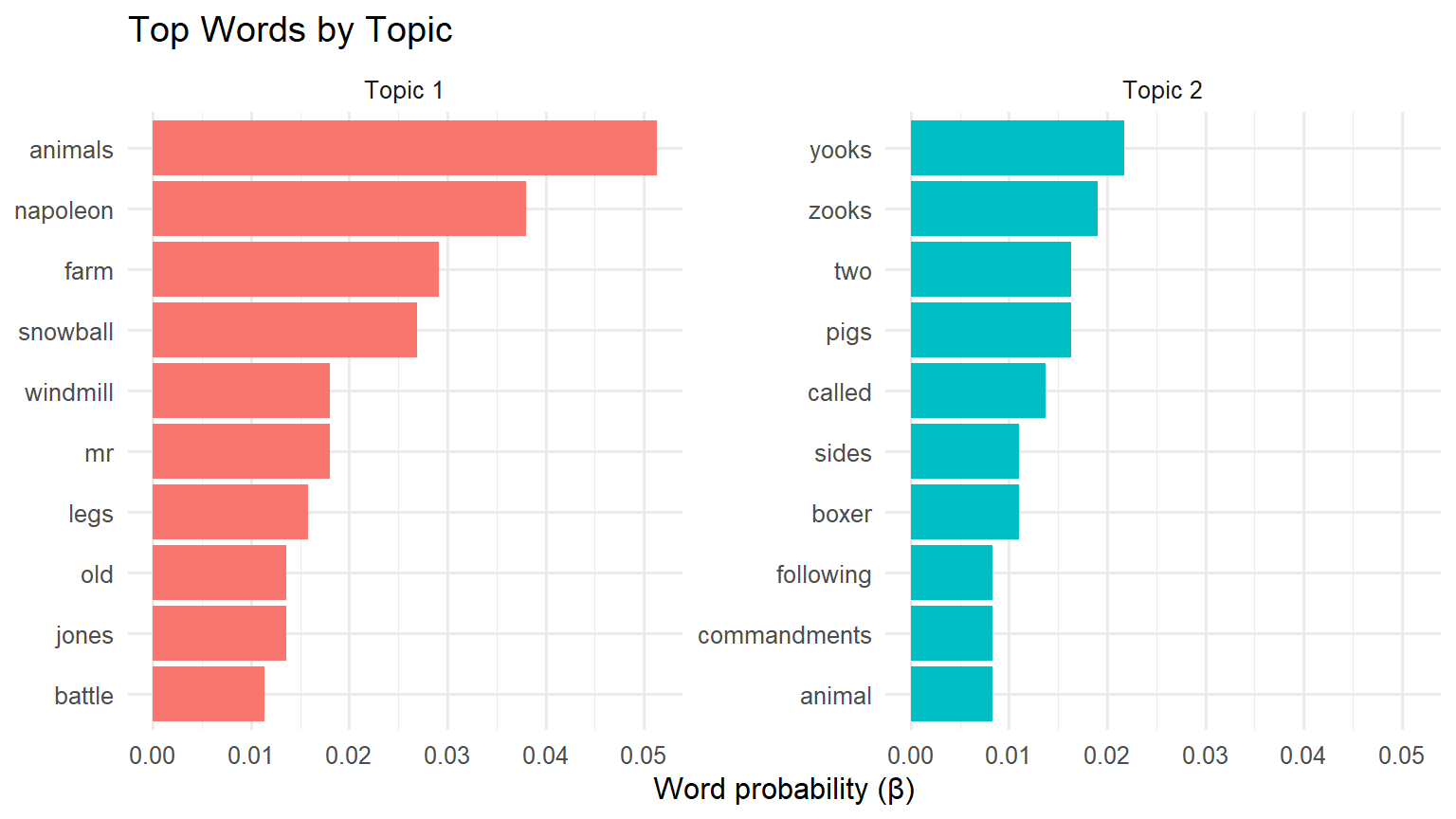
Figure 1: Top words in each topic (Animal Farm vs Butter Battle)
Interpreting the Results
Topic 1 top words: animals, napoleon, farm, snowball…
→ Animal Farm ✓
Topic 2 top words: yooks, zooks, wall, battle…
→ The Butter Battle Book ✓
LDA successfully separated the two sources—without being told which paragraphs came from which book.
Log-Ratio Visualization
Which words most distinguish the topics?
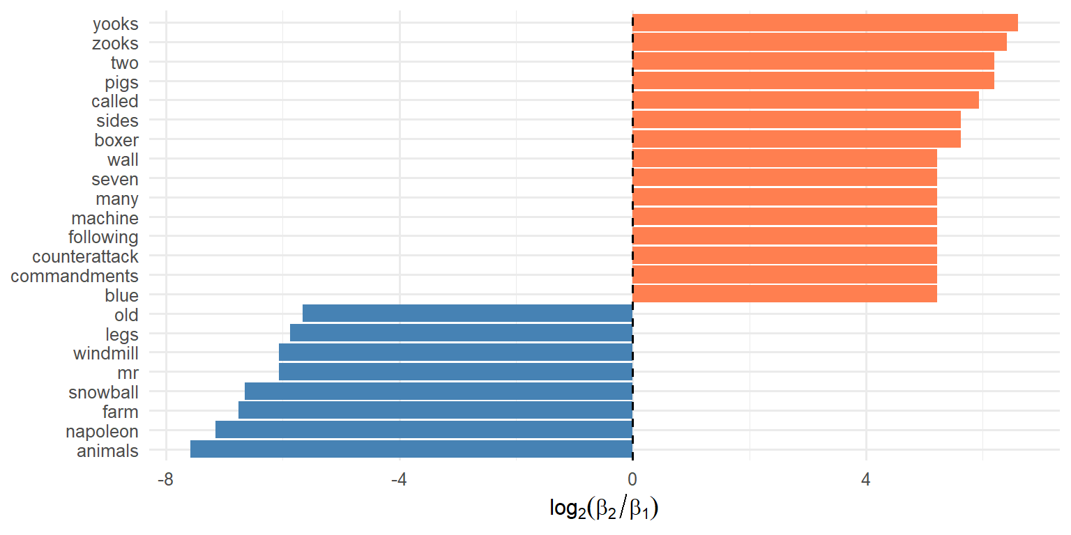
Figure 2: Log₂ ratio: positive = Topic 2 (Butter Battle), negative = Topic 1 (Animal Farm)
Toy Example: Takeaways
- LDA works: It found the two sources without supervision
- Interpretation requires judgment: “yooks” means nothing without context
- Limitations exposed: With only 9 documents (paragraphs), this is a toy. Real corpora have thousands of documents.
Let’s see what happens at scale.
Real Corpus: AP News
Associated Press Articles
2,246 news articles from the Associated Press.
In Chapter 10 we fit \(K = 2\) topics and found:
- Topic 1: Business/Finance
- Topic 2: Politics/Government
Now: What if we ask for \(K = 4\) topics?
Fitting LDA with K = 4
Four Topics Discovered
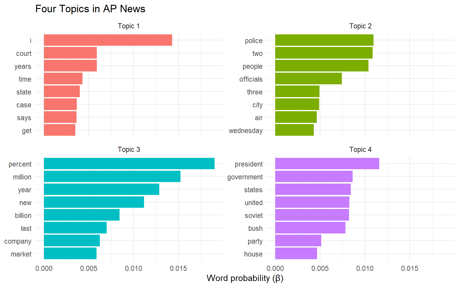
Figure 3: Top words in each of 4 topics (AP articles)
Interpreting the Four Topics
| Topic | Top Words | Interpretation |
|---|---|---|
| 1 | percent, million, market, stock | Business/Finance |
| 2 | president, government, party | Politics (Domestic) |
| 3 | soviet, united, states, military | International/Cold War |
| 4 | police, people, city, reported | Local News/Crime |
These interpretations require domain knowledge. The algorithm provides the word distributions; you provide the labels.
Topic Mixtures per Document \((\gamma)\)
Each document has a mixture of topics:
| Doc ID | Topic 1 | Topic 2 | Topic 3 | Topic 4 |
|---|---|---|---|---|
| 195 | 0.53 | 0.16 | 0.14 | 0.18 |
| 526 | 0.18 | 0.44 | 0.15 | 0.23 |
| 1842 | 0.12 | 0.62 | 0.13 | 0.13 |
| 2227 | 0.10 | 0.09 | 0.72 | 0.09 |
Most documents lean toward one topic, but more even mixtures are common.
Visualizing Document Mixtures
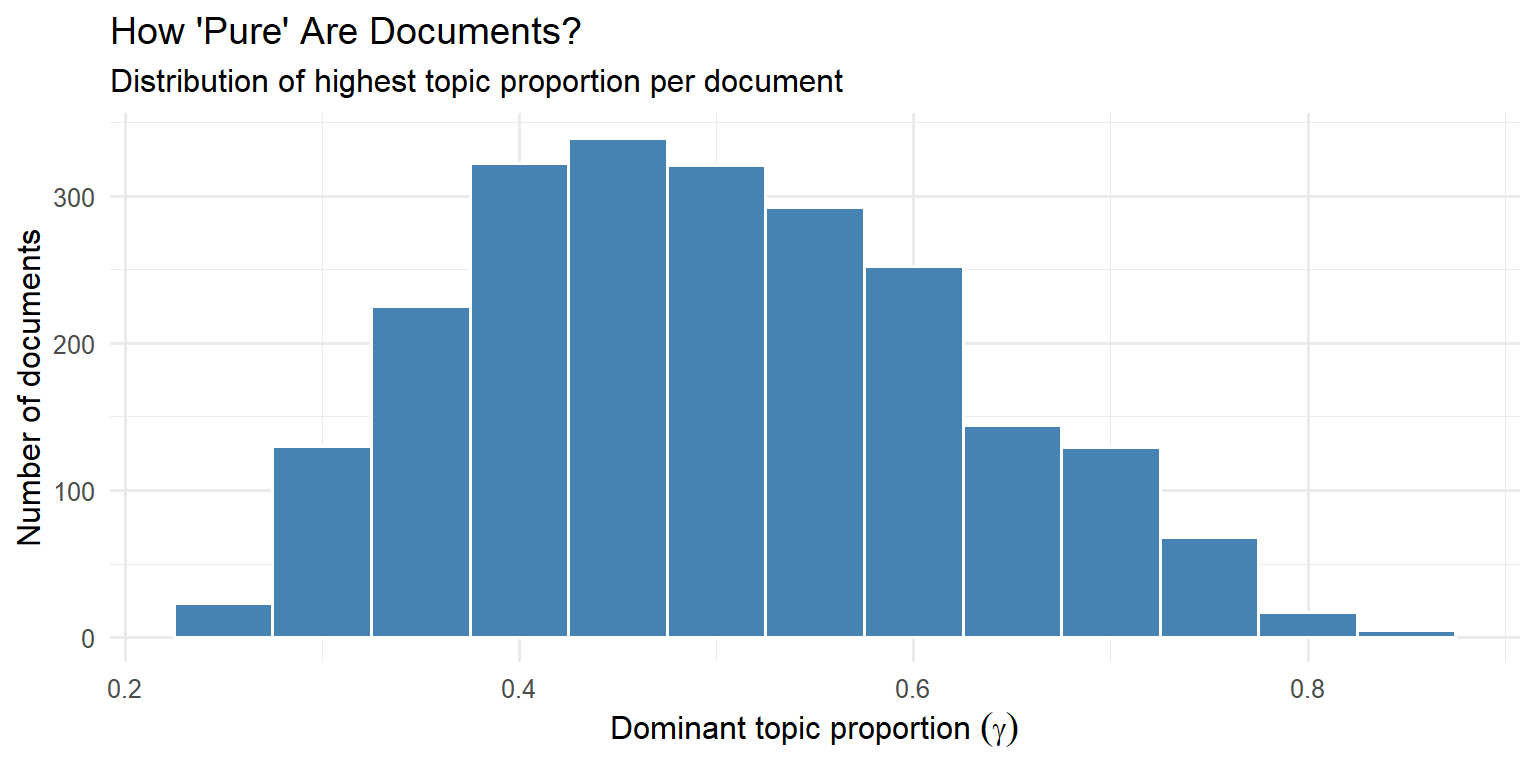
Figure 4: Distribution of dominant topic proportions
A few articles are dominated by one topic \((\gamma > 0.8)\), but most articles are a mixture of two or more topics.
The Dirichlet Distribution
Why “Dirichlet” in LDA?
LDA needs a probability distribution over mixtures.
- Each document has a particular mixture of topics
- The mixture is given as probability vector like (0.7, 0.3)
The Dirichlet distribution is a distribution over such probability vectors.
A Distribution Over Mixtures
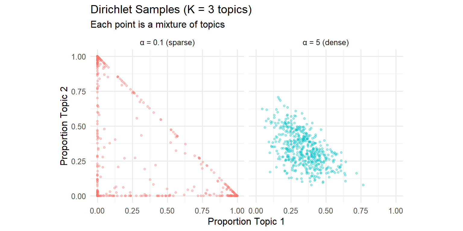
Samples from Dirichlet distributions with different concentrations
The Concentration Parameter
The Dirichlet has a concentration parameter \(\alpha\):
Small \(\alpha\) (< 1): Sparse mixtures
- Documents tend toward one dominant topic
- “This article is 95% politics”
Large \(\alpha\) (> 1): Uniform mixtures
- Documents spread across many topics
- “This article is 30% politics, 35% business, 35% international”
LDA typically uses small \(\alpha\), reflecting the intuition that documents are usually about something specific.
Dirichlet in the LDA Model
LDA uses two Dirichlet distributions:
- α controls topic mixtures per document \((\gamma)\)
- “How focused are documents on single topics?”
- β (sometimes called \(\delta\) or \(\eta\)) controls word mixtures per topic
- “How focused are topics on specific words?”
These are hyperparameters you can tune—but defaults often work well.
Choosing K
The Key Question
How many topics should you request?
This is analogous to choosing \(K\) in K-means clustering.
Too few topics: Themes are too broad
- Business and finance lumped together
- Important distinctions lost
Too many topics: Themes are too narrow
- Redundant topics
- Hard to interpret
No Perfect Answer
Unlike clustering, there’s no “elbow” method that works reliably.
Practical approaches:
- Domain knowledge: “I expect 5–10 themes in this corpus”
- Interpretability: Can you name each topic? Do the top words cohere?
- Iteration: Fit K = 2, 3, 5, 10. Compare results.
- Coherence metrics: Statistical measures of topic quality (advanced)
Example: K = 2 vs K = 4 vs K = 8
K = 2: i, people, two, president, government
K = 4: Splits into Business, Politics, International, Local
K = 8: Further splits may reveal Sports, Legal, Technology…
…or may produce redundant, uninterpretable topics.
Guidance for Choosing K
Practical Recommendations
- Start with domain intuition — How many themes do you expect?
- Try a range — e.g., K = 2, 3, 5, 10
- Evaluate interpretability — Can you name each topic?
- Look for redundancy — Do topics overlap too much?
- Consider your goal — Exploration (fewer topics) vs. fine-grained analysis (more topics)
Summary
Key Takeaways
- Topic models assume documents are mixtures of topics, and topics are mixtures of words
- LDA discovers both word distributions \((\beta)\) per topic and topic distributions \((\gamma)\) per document
- Interpretation requires judgment — the algorithm finds patterns; you provide meaning
- Choosing K is an art — iterate, evaluate, use domain knowledge
- The Dirichlet distribution provides the “mixture over mixtures” structure LDA needs
Key Notation
| Symbol | Meaning |
|---|---|
| \(K\) | Number of topics (you choose) |
| \(\alpha\) | Dirichlet concentration of topic mixtures per doc |
| \(\beta_{k,v}\) | Probability of term \(v\) in topic \(k\) |
| \(\gamma_{d,k}\) | Proportion of topic \(k\) in document \(d\) |
For each topic \(k\): \(\sum_v \beta_{k,v} = 1\)
For each document \(d\): \(\sum_k \gamma_{d,k} = 1\)
Connections to Earlier Material
| Earlier Concept | Topic Model Analog |
|---|---|
| K-means clustering | LDA (documents → topics) |
| Cluster centroids | Word mixtures (β) per topic |
| Cluster assignments | Topic mixtures (γ) per document |
| Choosing K | Choosing K |
| PCA loadings | Word weights per topic |
Topic models are “soft clustering” — documents belong partially to multiple topics.
The Two LDAs Resolved
Two Different Techniques
Linear Discriminant Analysis (Chapter 9)
- Supervised: uses class labels
- Finds directions that separate known classes
Latent Dirichlet Allocation (Chapter 11)
- Unsupervised: discovers latent structure
- Finds topics from word co-occurrence
Both “allocate” observations to categories—but with very different goals.
Exercises
Team Exercise 1: Interpret Topics
Using the AP News K = 4 results:
- Propose alternative labels for each topic. Justify with top words.
- Which topic is most coherent? Least coherent? Why?
- Find a word that appears in multiple topics. What does this suggest?
Team Exercise 2: Document Mixtures
For a document with \(\gamma = (0.4, 0.3, 0.2, 0.1)\):
- What does this mixture tell you about the document?
- How would you summarize this to a non-technical colleague?
- Would you classify this document into one topic or multiple? Why?
Team Exercise 3: Choosing K
You have a corpus of 5,000 customer support tickets.
- What K would you start with? Why?
- Design an evaluation process to compare different values of K.
- How would you explain your choice to stakeholders?
Team Exercise 4: LDA vs LLMs
For theme discovery in a large corpus:
- When would you prefer LDA over asking an LLM?
- When would you prefer an LLM over LDA?
- Design a hybrid workflow combining both approaches.
Resources
References
Foundational:
Blei, Ng, & Jordan (2003). Latent Dirichlet Allocation. JMLR.
Steyvers & Griffiths (2007). Probabilistic Topic Models. In Handbook of Latent Semantic Analysis.
Practical:
Silge & Robinson. Text Mining with R, Chapter 6.
Antoniak (2023). LDA in Practice. Blog post with practical advice.
R Functions Reference
| Function | Package | Purpose |
|---|---|---|
LDA() |
topicmodels | Fit LDA model |
tidy() |
tidytext | Extract β or γ matrices |
cast_dtm() |
tidytext | Create document-term matrix |
perplexity() |
topicmodels | Model fit metric |