Time Series Data

Two Lenses, One Reality

EDA for Machine Learning

The Nature of Time Series

Understanding and Prediction

Throughout this book we have seen that understanding and decision support are intertwined.

Time series analysis makes this especially vivid.

Domain Question
Time How does the past predict the future?
Frequency What structure generated this process?

These are not competing approaches—they are dual perspectives on the same underlying reality, connected by mathematics.

Time Series Have Memory

Standard assumption in statistics: Observations are independent

Time series reality: Successive observations are dependent

This dependence is not merely a technical nuisance. It is information:

  • Information about how the system evolves
  • Information about underlying periodic structure
  • Information we must understand to make correct inferences

Two Equivalent Descriptions

The dependence structure of a stationary time series has two equivalent descriptions:

Domain Object Question
Time Autocorrelation function \(\rho(u)\) How does \(X(t)\) correlate with \(X(t-u)\)?
Frequency Spectral density \(f(\lambda)\) How much variance comes from frequency \(\lambda\)?

These contain the same information—they are Fourier transform pairs.

Understanding both illuminates what either alone obscures.

Why Fourier Analysis Is Fundamental

This is not historical accident. There is a deep reason.

The back-shift operator \(\mathcal{B}\) shifts a process in time:

\[[\mathcal{B}X](t) = X(t-1)\]

Complex exponentials \(e_\lambda(t) = e^{i\lambda t}\) are eigenfunctions of \(\mathcal{B}\):

\[\mathcal{B}(e_\lambda) = e^{-i\lambda} \cdot e_\lambda\]

Sinusoids are the natural “modes” of any time-invariant linear system.

The Creation Myth

One way to think about stationary processes:

In the beginning: White noise—independent observations, no memory

Then: A linear, time-invariant filter acts on the white noise

Result: Autocorrelated output—the filter’s fingerprint

The spectrum tells you what the filter did.

The ACF tells you how the present relates to the past.

Examples: Two Perspectives

Example 1: Sunspots

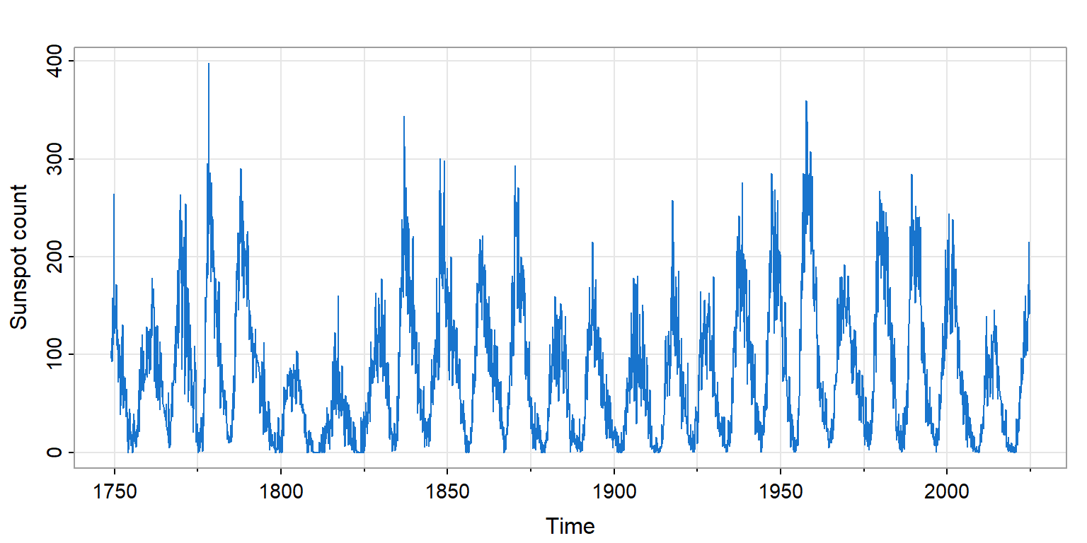
Figure 1: Monthly sunspot numbers, 1749–present

  • Visible structure: ~11-year solar magnetic cycle
  • Irregular amplitude: Peak heights vary substantially
  • What do the two lenses reveal?

Sunspots: Time Domain View
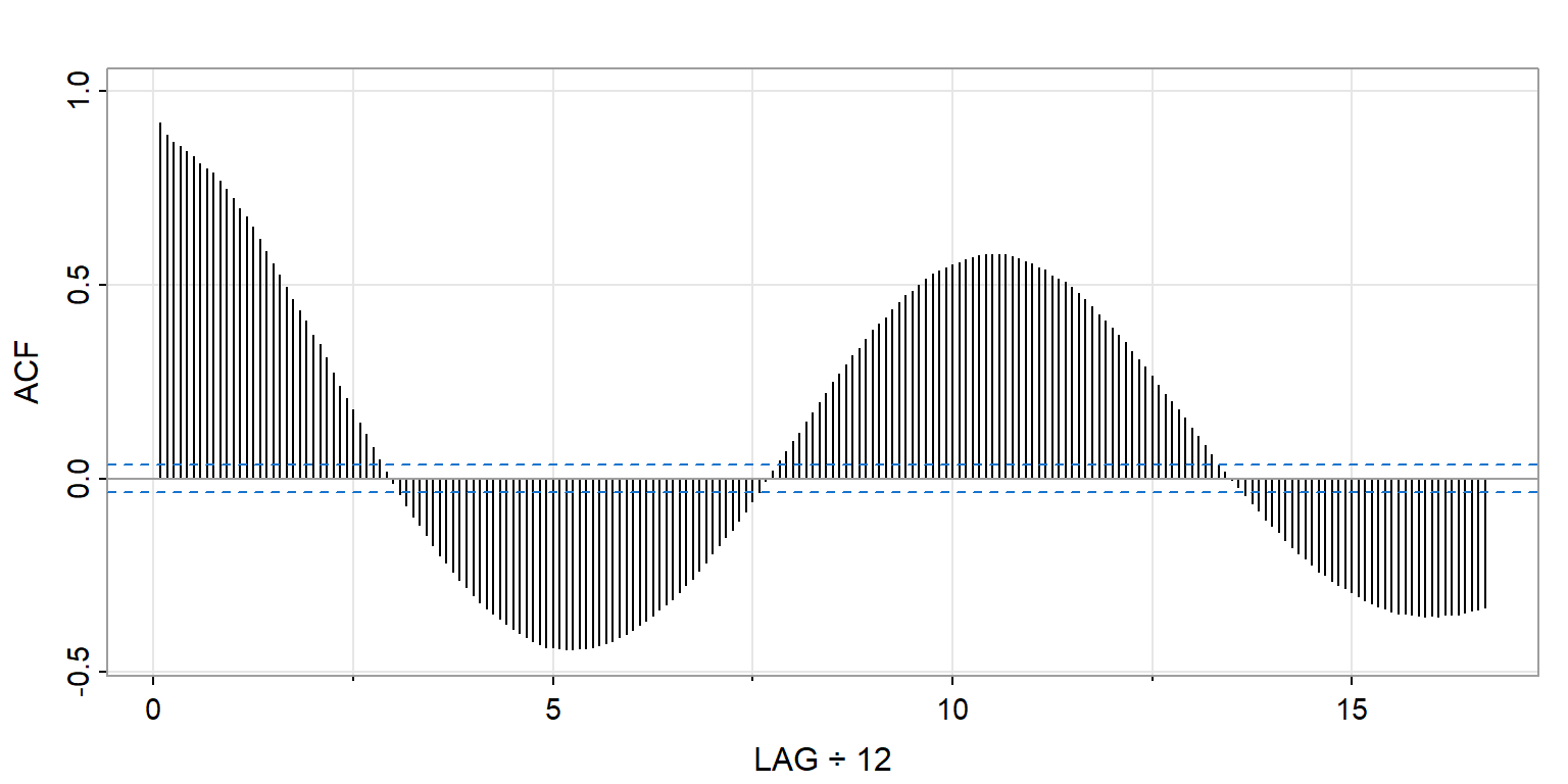
Figure 2: ACF of monthly sunspot numbers

  • Slow decay: Strong persistence—the past predicts the future
  • Oscillation: Cycle of ~11 years
  • But cycle length is hard to read precisely

Sunspots: Frequency Domain View
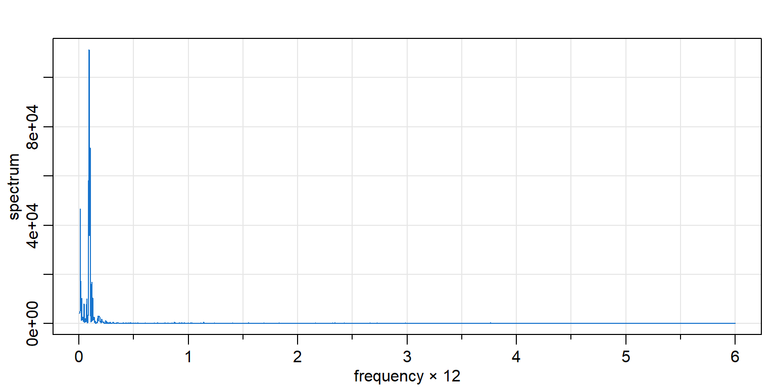
Figure 3: Spectrum of monthly sunspot numbers

  • Dominant peak: The ~11-year cycle appears as a sharp spectral peak
  • Frequency ≈ 0.007 cycles/month → period ≈ 140 months ≈ 11.7 years
  • The spectrum makes the periodicity immediately visible

Example 2: Global Temperatures
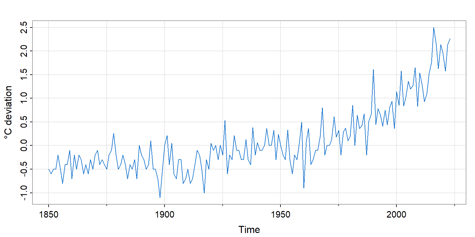
Figure 4: Annual temperature deviations from 1991–2020 average

  • Dominant feature: Non-linear trend, especially post-1980
  • No obvious periodicity: Unlike sunspots
  • How do the two lenses handle trend?

Global Temperatures: Time Domain
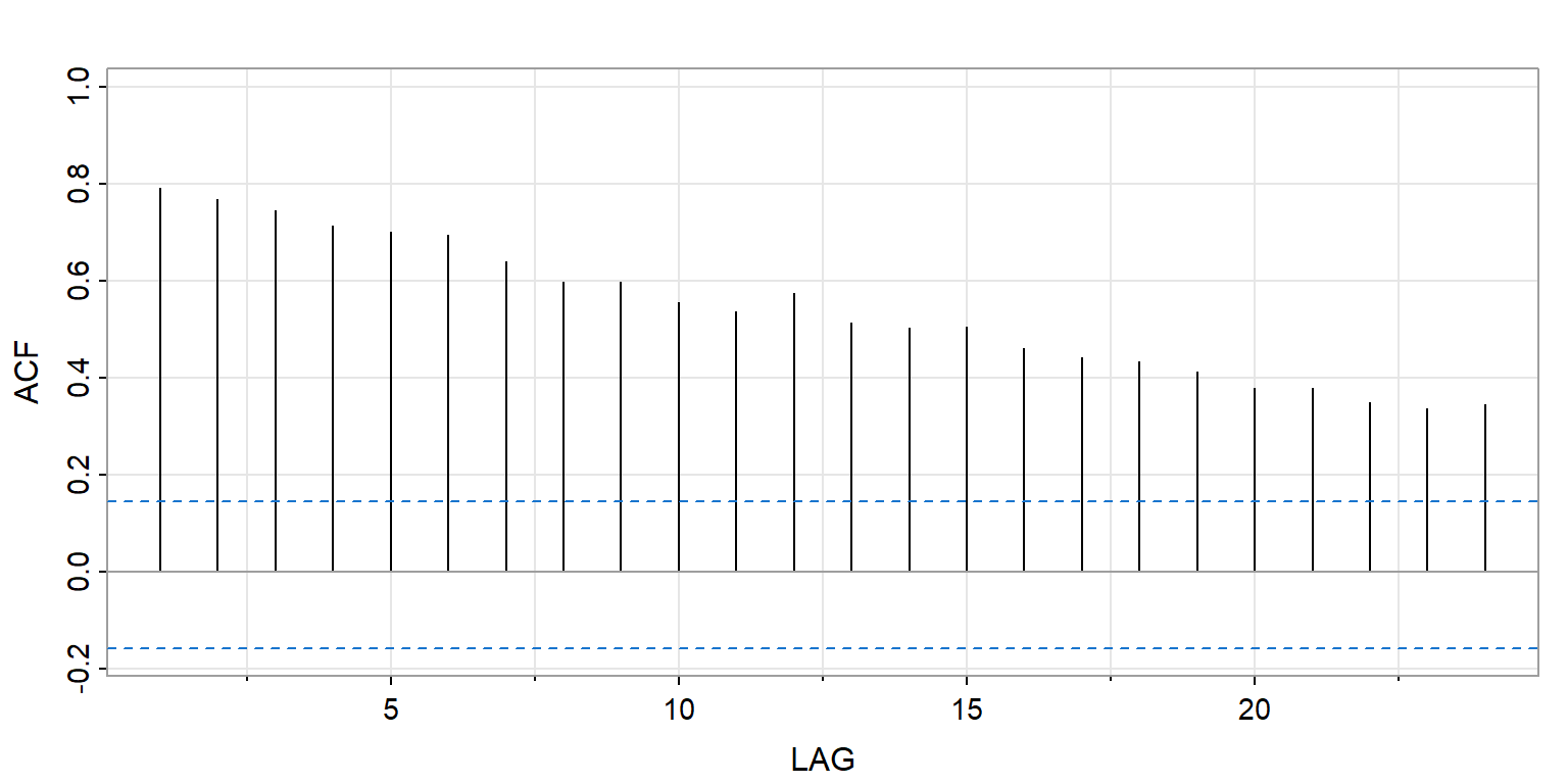
Figure 5: ACF of global land temperatures

  • Very slow decay: Each year strongly predicts the next
  • This signals non-stationarity—the trend dominates
  • Must remove trend before standard time series analysis

Global Temperatures: Frequency Domain
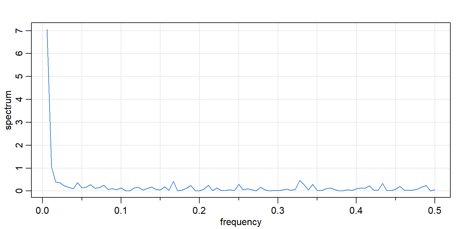
Figure 6: Spectrum of global land temperatures

  • Low-frequency dominance: Most variance at lowest frequencies
  • This is the spectral signature of trend
  • No periodic peaks—the story is secular change, not cycles

Example 3: SOI and Fish Recruitment
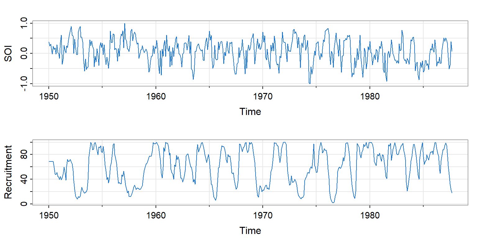
Figure 7: Southern Oscillation Index and Recruitment, 1950–1987

  • Two related series: Ocean temperature affects fish population
  • Multiple periodicities: Annual cycle + El Niño (~4 years)
  • Perfect case for spectral analysis

SOI: Dual Perspective
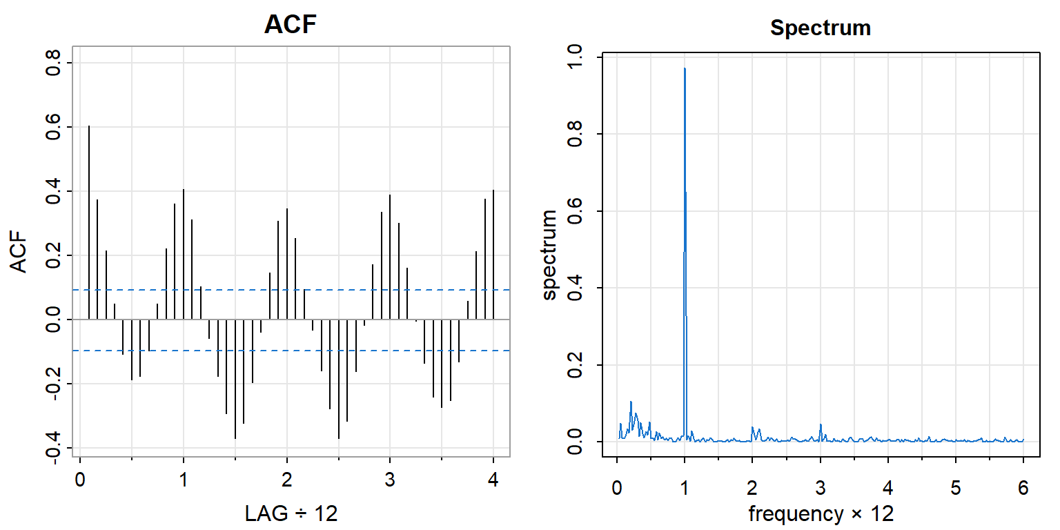
Figure 8: SOI: ACF and Spectrum

  • ACF: Oscillates, showing cyclical structure, but which cycles?
  • Spectrum: Two clear peaks—annual (freq ≈ 1) and El Niño (freq ≈ 0.25)
  • The frequency domain separates the periodicities

Recruitment: Dual Perspective
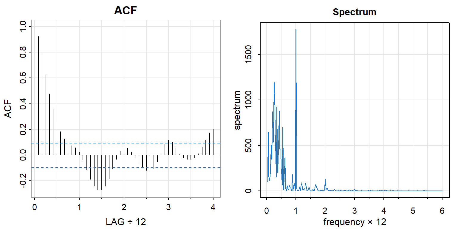
Figure 9: Recruitment: ACF and Spectrum

  • Similar spectral peaks to SOI—the fish respond to the climate signal
  • This correspondence leads to coherence analysis (Chapter 14)
  • Understanding the mechanism enables better forecasting

The White Noise Baseline

White Noise: The Blank Slate

White noise is the reference point—a process with no memory:

  • Independent observations
  • Constant variance
  • Zero autocorrelation at all nonzero lags

Time domain: \(\rho(u) = 0\) for all \(u \neq 0\)

Frequency domain: Flat spectrum—equal variance at all frequencies

White Noise: Visual Signature

Bandwidth: 0.072 | Degrees of Freedom: 72.12 | split taper: 0% 
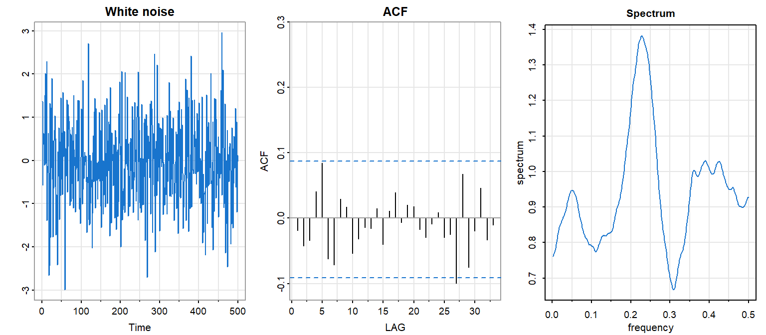
Figure 10: White noise: time series, ACF, and spectrum

  • Time series: No visible pattern
  • ACF: All lags near zero (within confidence bands)
  • Spectrum: Flat (within confidence bands)—no frequency dominates

Departures from White Noise

Any structure in ACF or spectrum reveals departure from independence:

Observation Time Domain Frequency Domain
Slow ACF decay Persistence/trend Low-freq dominance
ACF oscillation Cyclical dependence Spectral peaks
Sharp ACF cutoff Short memory (MA) Smooth spectrum
Gradual ACF decay Long memory (AR) Peaked spectrum

The two views are complementary diagnostics.

Stationarity and Time-Invariance

Stationarity Defined

A process is second-order stationary (weakly stationary) if:

  1. \(E\{X(t)\} = \mu\) (constant mean)

  2. \(\text{Cov}(X(t+u), X(t)) = \gamma(u)\) (depends only on lag \(u\))

Why it matters:

  • Stationarity lets us estimate \(\gamma(u)\) from a single realization
  • The spectrum is only defined for stationary processes
  • Non-stationary series must be transformed first

Stationarity and Time-Invariance

Stationarity is the statistical counterpart of time-invariance in systems theory.

A linear filter is time-invariant if shifting the input shifts the output by the same amount—the filter doesn’t care what time it is.

Stationary processes are precisely those whose statistical properties don’t care what time it is.

This connection is why Fourier methods—natural for time-invariant systems—are fundamental for stationary processes.

Stationarity: Visual Assessment

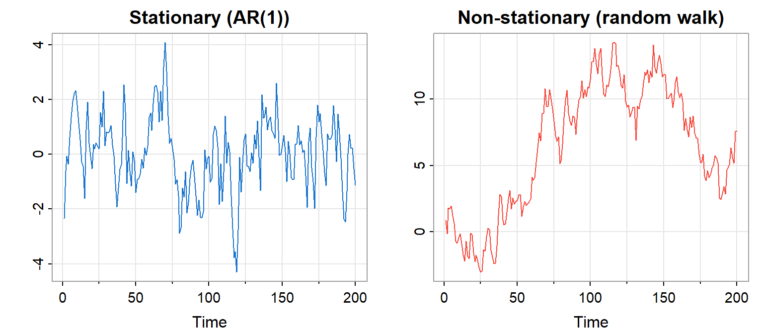
Figure 11: Stationary vs. non-stationary

  • Left: Fluctuates around a constant level—stationary
  • Right: Wanders without returning—non-stationary

Achieving Stationarity

Common transformations for non-stationary data:

Problem Transformation
Trend in mean Differencing: \(Y(t) = X(t) - X(t-1)\)
Exponential growth Log transform, then difference
Changing variance Log or Box-Cox transform
Seasonality Seasonal differencing

After transformation, check that ACF decays and spectrum is not dominated by lowest frequencies.

Autocorrelation in Detail

The Autocorrelation Function

\[\rho_X(u) = \frac{\gamma_X(u)}{\gamma_X(0)} = \text{Corr}(X(t+u), X(t))\]

Properties:

  • \(\rho_X(0) = 1\) (perfect self-correlation)
  • \(|\rho_X(u)| \leq 1\) (it’s a correlation)
  • \(\rho_X(-u) = \rho_X(u)\) (symmetric in lag)

The ACF answers: How predictable is the future from the past?

Sample ACF

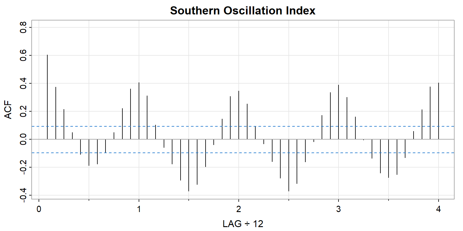
Figure 12: Sample ACF for SOI data

  • Blue dashed lines: 95% confidence bounds under white noise null
  • Values outside bounds → significant autocorrelation
  • Pattern of decay/oscillation suggests model structure

Partial Autocorrelation Function (PACF)

The PACF measures correlation between \(X(t+u)\) and \(X(t)\) after removing the linear effect of intervening values.

\[\phi_{uu} = \text{Corr}(X(t+u) - \hat{X}(t+u), \; X(t) - \hat{X}(t))\]

The PACF answers: What is the direct effect of lag \(u\), controlling for shorter lags?

ACF and PACF Together

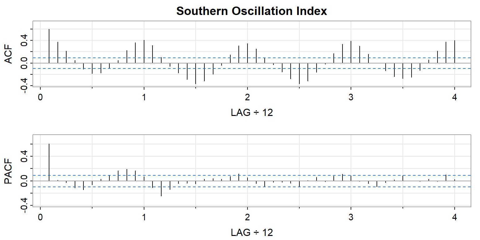
Figure 13: ACF and PACF for SOI data

  • ACF: Total correlation at each lag
  • PACF: Direct effect at each lag, controlling for others
  • Together they suggest model structure (Chapter 13)

Why Correct Inference Requires Understanding

The Variance Problem

Suppose we estimate the mean \(\mu_X\) from \(T\) observations.

If independent: \[\text{Var}(\bar{X}) = \frac{\sigma_X^2}{T}\]

If autocorrelated: \[\text{Var}(\bar{X}) = \frac{\sigma_X^2}{T} \left(1 + 2\sum_{u=1}^{T-1}\left(1 - \frac{u}{T}\right)\rho_X(u)\right)\]

Ignoring autocorrelation gives wrong standard errors.

This is a failure of understanding producing a failure of inference.

Effective Sample Size

Question: How many independent observations would give the same variance?

\[N_{\text{eff}} = \frac{T}{\displaystyle 1 + 2\sum_{u=1}^{T-1}\left(1 - \frac{u}{T}\right)\rho_X(u)}\]

Example: If \(\rho_X(1) = 0.8\) and higher lags decay geometrically…

  • \(T = 100\) observations
  • \(N_{\text{eff}} \approx 11\) effective observations

Your sample is 9× smaller than it appears!

Practical Consequences

If you ignore autocorrelation… Consequence
Confidence intervals Too narrow
Hypothesis tests Too many false positives
Standard errors Underestimated
Cross-validation Training/test not independent

The lesson: Understanding the dependence structure is essential for valid inference.

This is not merely academic—it affects real decisions.

Looking Ahead

Two Chapters, Two Emphases

Chapter 13: Time Domain Methods

  • ARIMA models: AR, MA, and their combinations
  • Forecasting and prediction intervals
  • Emphasis: predicting the future from the past

Chapter 14: Frequency Domain Methods

  • Periodogram and spectral density estimation
  • Coherence between series
  • Emphasis: understanding periodic structure

Both perspectives are needed for complete understanding.

The Dual Aims, Revisited

Time series analysis embodies the dual aims of data analysis:

Decision support: Forecast tomorrow’s value, next quarter’s earnings, next year’s climate

Scientific understanding: What periodic phenomena drive the system? What filtering has occurred? What is the physics?

Effective forecasting rests on understanding; understanding is tested by predictive success.

The two aims are inseparable.

Summary

Key Insights

  1. Time series have memory—the present depends on the past

  2. Two equivalent descriptions: ACF (time domain) and spectrum (frequency domain)

  3. Fourier analysis is fundamental because sinusoids are eigenfunctions of time-shift

  4. Stationarity is the statistical counterpart of time-invariance

  5. Ignoring structure invalidates inference—ESS reveals your true sample size

  6. Understanding and prediction are intertwined—the dual aims made precise

Diagnostic Checklist

When you encounter a new time series:

  1. Plot the series: Look for trend, seasonality, level shifts, changing variance

  2. Check stationarity: Does \(X\) wander? Transform as needed

  3. Examine the ACF: How fast does it decay? Any oscillation?

  4. Examine the spectrum: Any dominant peaks? Low-frequency dominance?

  5. Consider ESS: How much independent information do you really have?

  6. Ask both questions: What predicts the future? What structure is present?

Exercises

Team Exercise 1: Explore an astsa Dataset

Choose a time series from astsa not discussed today (e.g., nyse, oil, prodn):

  1. Plot the series. What features do you observe?
  2. Plot the ACF. Is there evidence of autocorrelation?
  3. Does the series appear stationary? What would you do if not?

Team Exercise 2: Simulate White Noise

Generate 500 observations of Gaussian white noise using rnorm():

  1. Plot the series, ACF, and spectrum.
  2. How do they compare to theoretical signatures (flat spectrum, ACF = 0 at all lags)?
  3. Repeat several times. How much sampling variation do you see?

Team Exercise 3: Effective Sample Size

For an AR(1) process, \(ESS \approx T \cdot (1 - \phi) / (1 + \phi)\).

  1. Calculate ESS for \(T = 200\) when \(\phi = 0.5\), \(0.8\), \(0.95\).
  2. What happens as \(\phi \to 1\)?
  3. You have \(T = 100\) observations with estimated \(\phi = 0.7\). How wide should your confidence interval for the mean be, compared to the naive interval?

Discussion Questions

  1. You fit a regression and the residuals have ACF(1) = 0.4. What are the implications?

  2. When is first differencing appropriate? When might it remove too much signal?

  3. “The spectrum and ACF contain the same information.” True in theory—why might one be more useful in practice?