| Step | Action |
|---|---|
| 1. Plot | Examine series for trend, seasonality, variance changes |
| 2. Transform | Difference or transform to achieve stationarity |
| 3. Identify | Use ACF/PACF to suggest model order |
| 4. Estimate | Fit candidate models; compare via AIC/BIC |
| 5. Diagnose | Check residuals: should look like white noise |
Time Domain Methods
ARIMA Models and Forecasting
EDA for Machine Learning
The Forecasting Problem
From Understanding to Prediction
Chapter 12 established that time series have memory—the present depends on the past.
Now we exploit that dependence for forecasting:
Given observations up to the present, what should we expect tomorrow, next quarter, next year?
This is the archetypal decision-support application of time series analysis.
The Central Question
\[\hat{X}(t_f + h) = \; ?\]
Given observations \(X(t_0), X(t_0+1), \ldots, X(t_f)\), predict the value \(h\) steps ahead.
Key insight: The autocorrelation structure tells us how to weight past observations.
- Strong recent dependence → recent values matter most
- Periodic structure → values from the same season matter
- Long memory → distant past still informative
Building Blocks
All time domain models build from these components:
| Component | Role |
|---|---|
| White noise \(W(t)\) | Independent shocks; the baseline |
| Back-shift \(\mathcal{B}\) | \(\mathcal{B}X(t) = X(t-1)\) |
| Differencing \(\nabla\) | \(\nabla = 1 - \mathcal{B}\) removes trend |
| AR polynomial \(\phi(\mathcal{B})\) | Autoregressive structure |
| MA polynomial \(\theta(\mathcal{B})\) | Moving average structure |
The art is combining these to capture the dependence structure revealed by ACF and PACF.
Autoregressive Models
AR(1): The Simplest Memory
An AR(1) process:
\[X(t) = \phi_1 X(t-1) + W(t)\]
The current value is a fraction of the previous value, plus a random shock.
Constraints:
- \(|\phi_1| < 1\) ensures stationarity
- \(\phi_1 > 0\): positive dependence (most common)
- \(\phi_1 < 0\): alternating pattern
AR(1): ACF and PACF
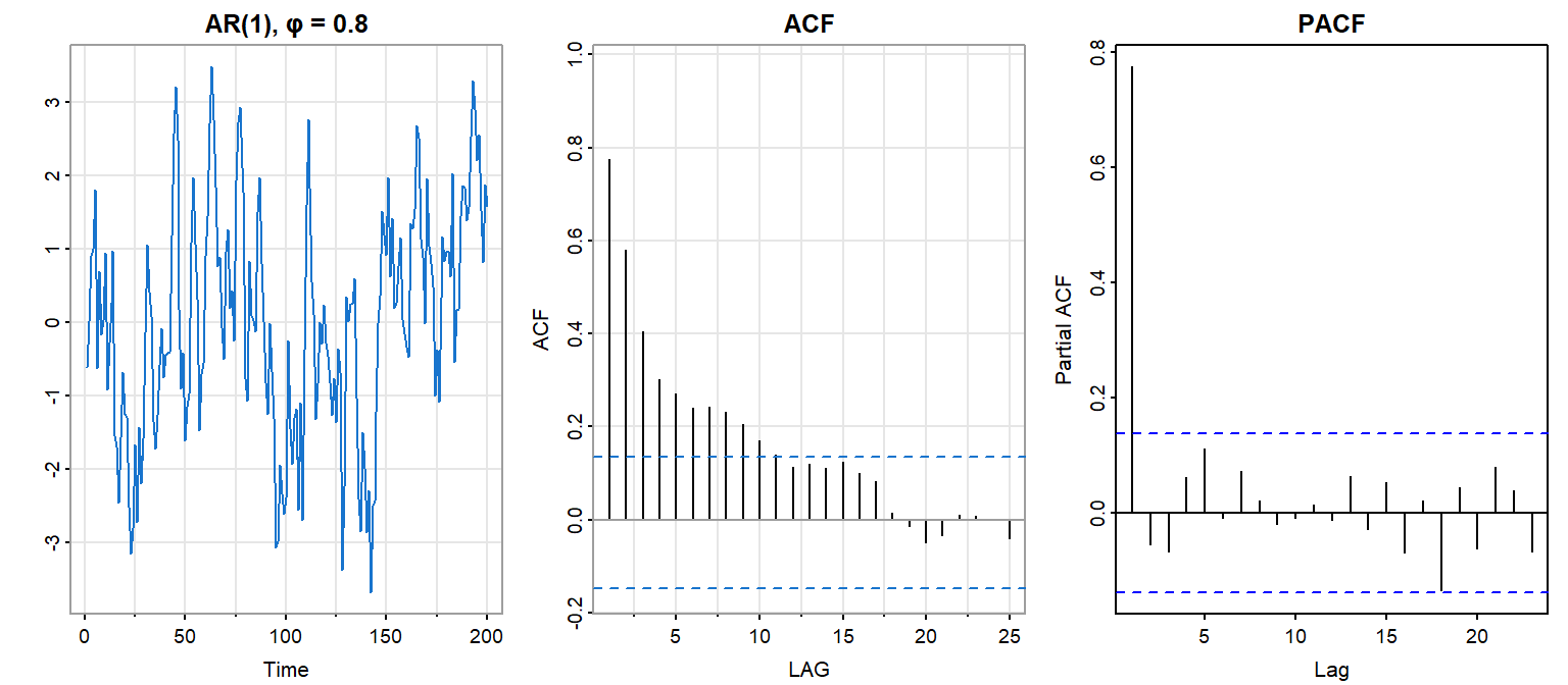
Figure 1: Simulated AR(1) with φ = 0.8
- ACF: Geometric decay \(\rho(h) = \phi_1^{|h|}\)
- PACF: Cuts off after lag 1
AR(1): The Signature
\[\rho_X(h) = \phi_1^{|h|}\]
The autocorrelation at lag \(h\) is the AR coefficient raised to the \(|h|\) power.
PACF: \[\phi_{hh} = \begin{cases} \phi_1 & h = 1 \\ 0 & h > 1 \end{cases}\]
The PACF cuts off after lag 1—this is the diagnostic signature of AR(1).
AR(p): Longer Memory
An AR(p) process depends on \(p\) past values:
\[X(t) = \phi_1 X(t-1) + \phi_2 X(t-2) + \cdots + \phi_p X(t-p) + W(t)\]
Polynomial form: \[\phi(\mathcal{B})(X(t) - \mu) = W(t)\]
where \(\phi(z) = 1 - \phi_1 z - \phi_2 z^2 - \cdots - \phi_p z^p\)
AR(p): Diagnostic Signature
| Feature | AR(p) Pattern |
|---|---|
| ACF | Decays gradually (exponential or damped oscillation) |
| PACF | Cuts off after lag \(p\) |
The PACF cutoff identifies the order. If you see that PACF is significant at lags 1 through \(p\) and near zero thereafter, consider an AR(p) model.
AR(2) Example: Recruitment
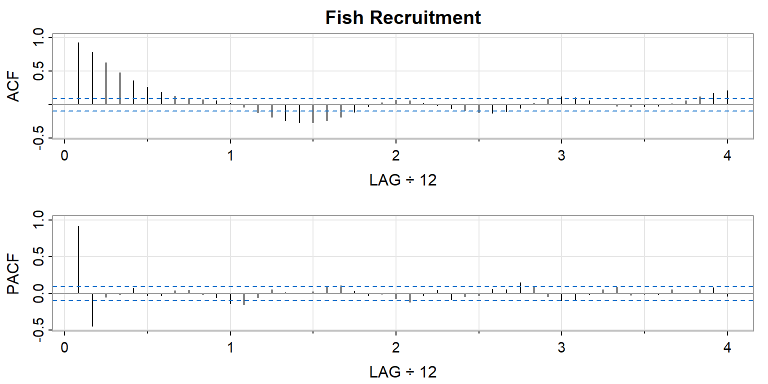
Figure 2: Recruitment data: ACF and PACF suggest AR(2)
- ACF shows damped oscillation (decays gradually)
- PACF has significant values at lags 1 and 2, then cuts off
- This pattern suggests AR(2)
Moving Average Models
MA(1): Dependence Through Shocks
An MA(1) process:
\[X(t) = W(t) + \theta_1 W(t-1)\]
The current value depends on the current shock and the previous shock.
Key difference from AR:
- AR: infinite memory (geometric decay)
- MA: finite memory (sharp cutoff)
MA(1): ACF and PACF
The autocorrelation structure:
\[\rho_X(h) = \begin{cases} 1 & h = 0 \\ \frac{\theta_1}{1 + \theta_1^2} & h = \pm 1 \\ 0 & |h| > 1 \end{cases}\]
| Feature | MA(1) Pattern |
|---|---|
| ACF | Cuts off after lag 1 |
| PACF | Decays gradually |
The opposite of AR(1)!
MA(q): The General Case
An MA(q) process:
\[X(t) = W(t) + \theta_1 W(t-1) + \cdots + \theta_q W(t-q)\]
Polynomial form: \[X(t) - \mu = \theta(\mathcal{B}) W(t)\]
where \(\theta(z) = 1 + \theta_1 z + \cdots + \theta_q z^q\)
Diagnostic signature: ACF cuts off after lag \(q\); PACF decays.
Invertibility
Problem: Different MA models can produce identical distributions.
Example: These two MA(1) processes are indistinguishable:
\[ \begin{align} X(t) &= W(t) + 0.2 W(t-1) & \sigma_W^2 = 25 \\ \\ Y(t) &= V(t) + 5 V(t-1) & \sigma_V^2 = 1 \end{align} \]
Solution: Require invertibility—all roots of \(\theta(z)\) outside the unit circle.
This ensures a unique representation and allows expressing \(W(t)\) in terms of past \(X\) values.
The Diagnostic Fingerprint
ACF vs PACF: The Key Patterns
| Model | ACF | PACF |
|---|---|---|
| AR(p) | Decays gradually | Cuts off after lag \(p\) |
| MA(q) | Cuts off after lag \(q\) | Decays gradually |
| ARMA(p,q) | Decays gradually | Decays gradually |
| White noise | All ≈ 0 | All ≈ 0 |
The identification strategy:
- If PACF cuts off → AR
- If ACF cuts off → MA
- If both decay → ARMA (or consider differencing)
Visual Guide: AR Signatures
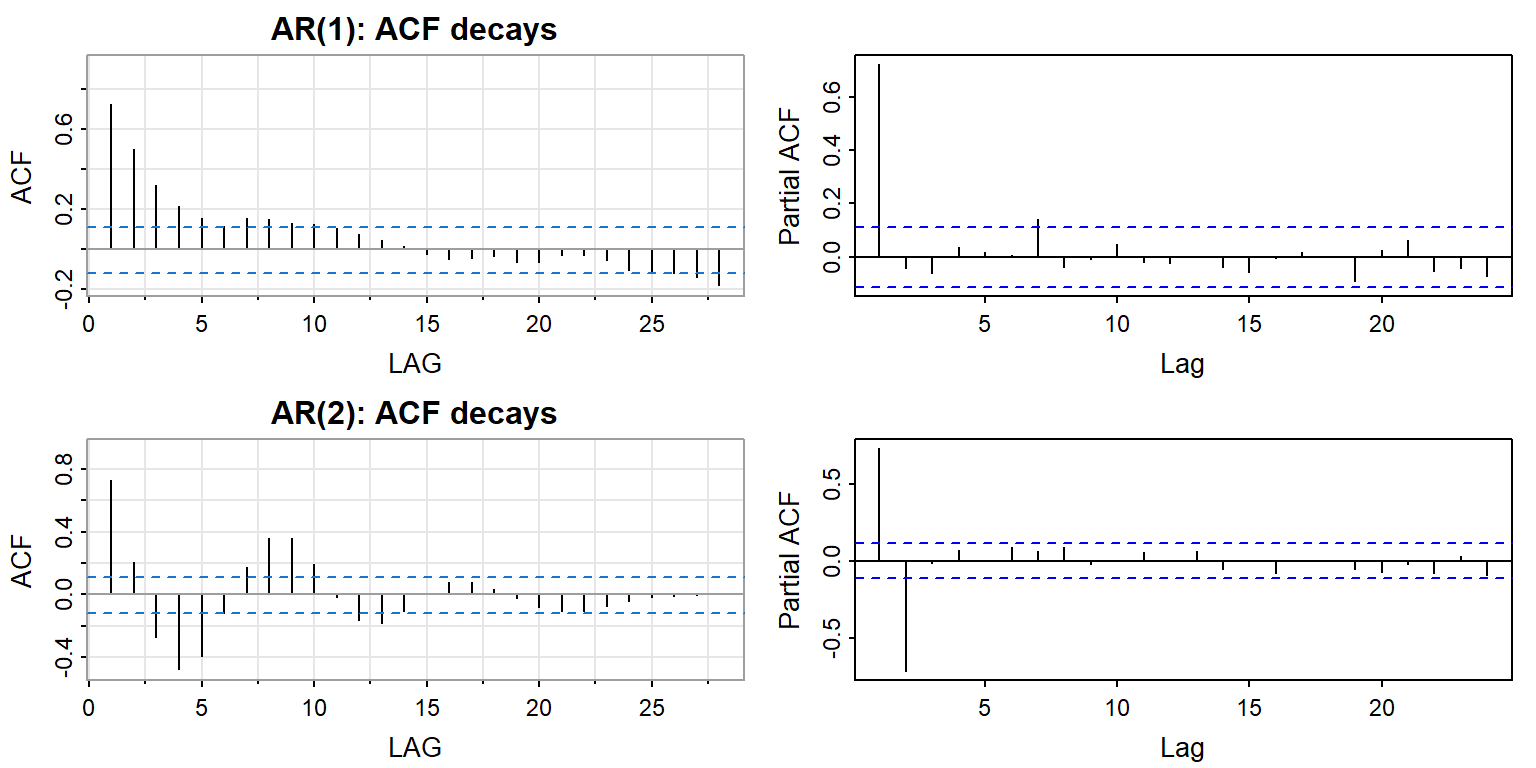
Figure 3: AR(1) and AR(2) signatures
Visual Guide: MA Signatures
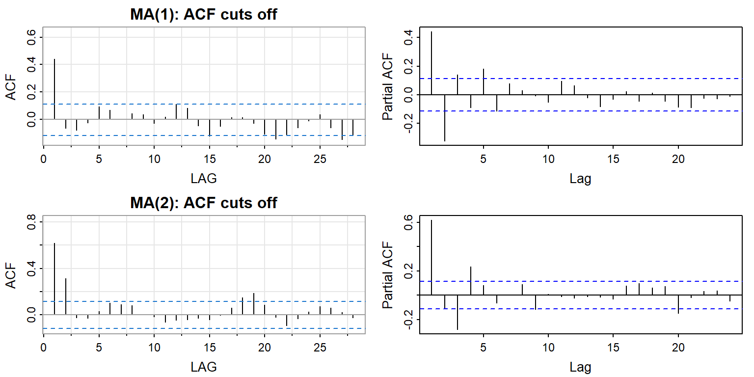
Figure 4: MA(1) and MA(2) signatures
ARMA Models
Combining AR and MA
An ARMA(p,q) process:
\[\phi(\mathcal{B})(X(t) - \mu) = \theta(\mathcal{B}) W(t)\]
Expanded: \[X(t) = \mu + \sum_{j=1}^{p} \phi_j (X(t-j) - \mu) + W(t) + \sum_{k=1}^{q} \theta_k W(t-k)\]
Why combine? Parsimony—a low-order ARMA may capture structure that would require high-order pure AR or MA.
ARMA: Two Representations
Causal form (as filtered white noise): \[X(t) - \mu = \sum_{\nu=0}^{\infty} \psi_\nu W(t-\nu)\]
Inverted form (white noise as filtered \(X\)): \[W(t) = \sum_{\nu=0}^{\infty} \pi_\nu (X(t-\nu) - \mu)\]
Both representations exist when AR and MA polynomials have roots outside the unit circle.
ARMA Diagnostics
For ARMA(p,q):
- ACF: Decays gradually (mixture of exponential and/or damped sinusoid)
- PACF: Decays gradually
Identification challenge: Both decay, so order selection is less clear.
Practical approach:
- Try to identify if pure AR or MA fits (check for cutoffs)
- If both decay, consider low-order ARMA(1,1) or ARMA(2,1)
- Use information criteria (AIC, BIC) to compare models
Non-Stationary Models
The Problem with Trends
Many real series are non-stationary:
- Global temperatures: upward trend
- Stock prices: random walk behavior
- Economic series: growth over time
The ACF and PACF diagnostics assume stationarity.
Solution: Transform to stationarity, then model.
Differencing Removes Trend
The differencing operator: \[\nabla X(t) = X(t) - X(t-1) = (1 - \mathcal{B})X(t)\]
If \(X(t)\) has a linear trend \(\mu + \beta t\): \[E\{\nabla X(t)\} = \beta \quad \text{(constant)}\]
Higher-order differencing \(\nabla^d\) removes polynomial trends of degree \(d\).
ARIMA(p, d, q)
An ARIMA(p, d, q) model:
\[\phi(\mathcal{B}) \nabla^d X(t) = \theta(\mathcal{B}) W(t)\]
- \(d = 0\): stationary ARMA
- \(d = 1\): first differences are ARMA (handles linear trend, random walk)
- \(d = 2\): second differences are ARMA (handles quadratic trend)
The “I” stands for Integrated—we integrate (cumsum) the ARMA process to get \(X(t)\).
Random Walk with Drift
A fundamental non-stationary model:
\[X(t) = \alpha + X(t-1) + W(t)\]
This is ARIMA(0, 1, 0) with drift \(\alpha\).
Properties:
- \(\nabla X(t) = \alpha + W(t)\) (differenced series is white noise + constant)
- Variance grows linearly with time
- Forecast: straight line from last observation with slope \(\alpha\)
Random Walk Forecast
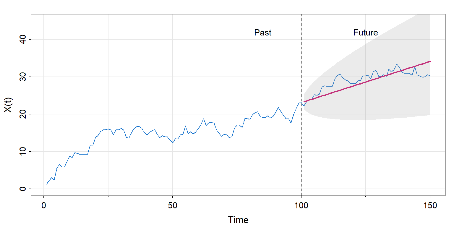
Figure 5: Random walk with drift: forecast is a ray
Prediction intervals widen with forecast horizon—uncertainty grows.
Seasonal Models
Seasonality in Time Series
Many series have periodic patterns:
- Monthly data: annual cycle
- Quarterly data: seasonal business patterns
- Daily data: weekly patterns
Seasonal differencing removes the periodic component:
\[\nabla_s X(t) = X(t) - X(t-s)\]
where \(s\) is the seasonal period (e.g., \(s = 12\) for monthly data).
SARIMA Models
A SARIMA model combines:
- Non-seasonal ARIMA(p, d, q)
- Seasonal ARIMA(P, D, Q)\(_s\)
\[\phi(\mathcal{B})\Phi(\mathcal{B}^s) \nabla^d \nabla_s^D X(t) = \theta(\mathcal{B})\Theta(\mathcal{B}^s) W(t)\]
Notation: ARIMA\((p,d,q) \times (P,D,Q)_s\)
CO₂ Example: Trend + Season
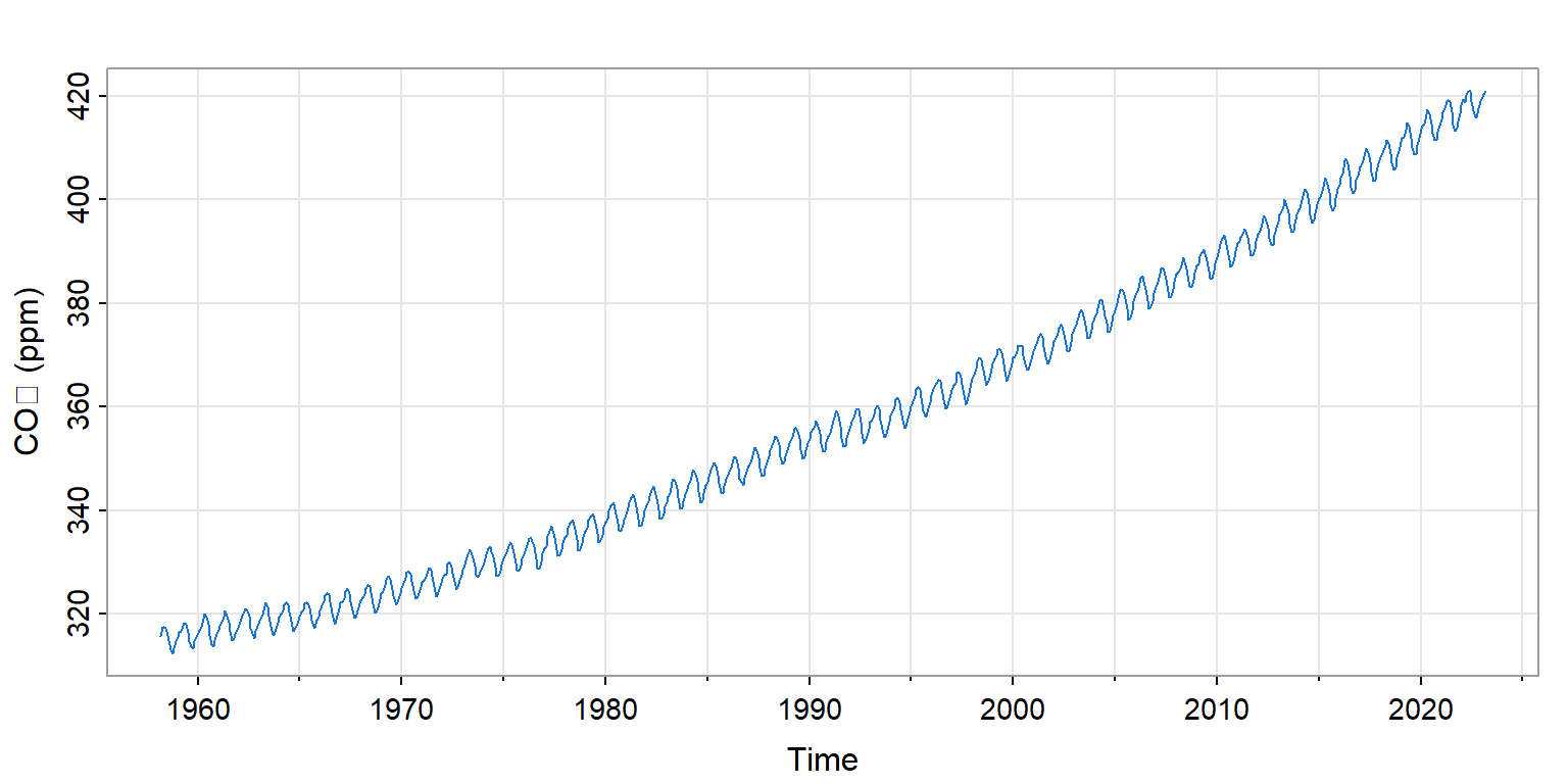
Figure 6: Mauna Loa CO₂: strong trend and annual cycle
This series needs both:
- Regular differencing (\(d = 1\)) for the trend
- Seasonal differencing (\(D = 1\), \(s = 12\)) for the annual cycle
CO₂: After Differencing
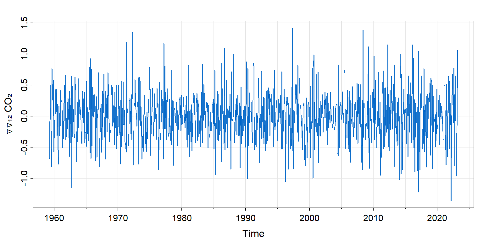
Figure 7: CO₂ after ∇∇₁₂: approximately stationary
After both differencing operations, the series appears stationary—ready for ARMA modeling.
CO₂: SARIMA Forecast
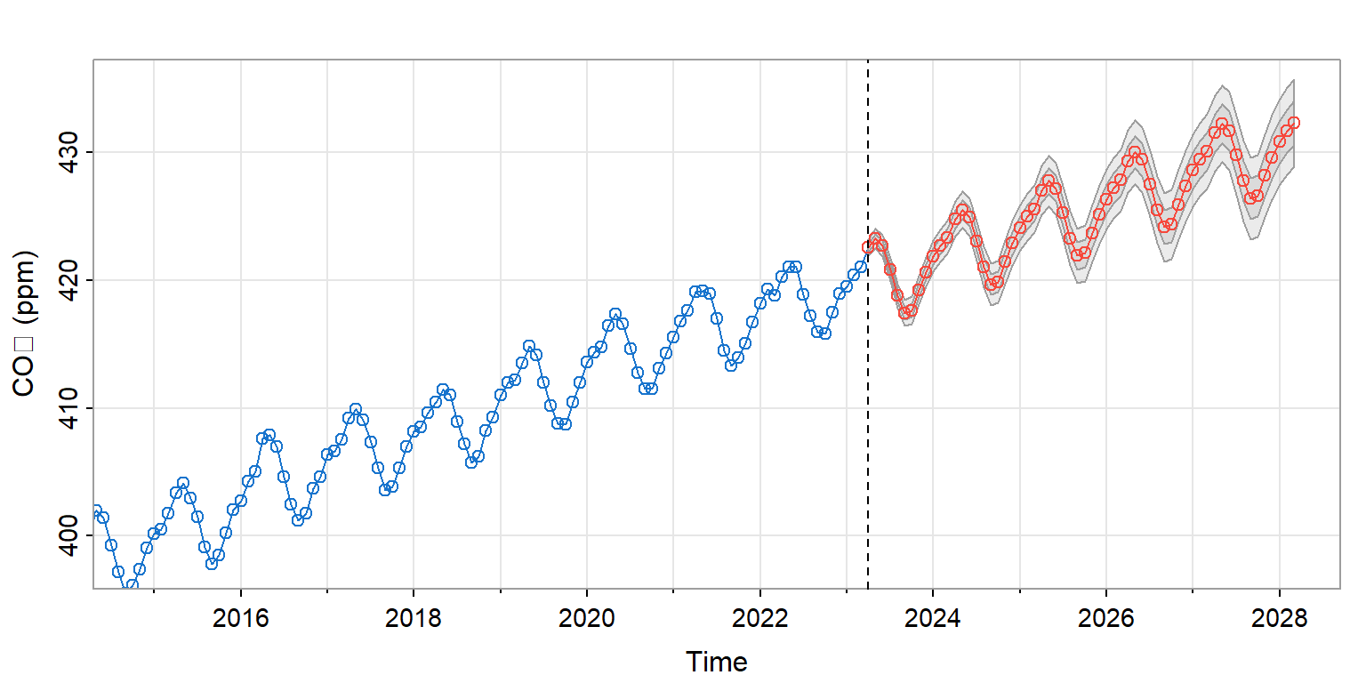
Figure 8: Five-year forecast from ARIMA(1,1,1)×(0,1,1)₁₂
The forecast captures both the upward trend and the seasonal oscillation.
Forecasting
The Linear Predictor
The best linear predictor of \(X(t_f + h)\) given the past:
\[\hat{X}(t_f + h) = \alpha + \sum_{\nu=0}^{T-1} \beta_\nu X(t_0 + \nu)\]
The coefficients \(\beta_\nu\) are chosen to minimize mean squared prediction error:
\[MSE = E\{(X(t_f + h) - \hat{X}(t_f + h))^2\}\]
ARMA Forecasting
For an ARMA process, the predictor has a simple recursive form.
One step ahead (\(h = 1\)): \[\hat{X}(t_f + 1) = \sum_{j=1}^{p} \phi_j X(t_f + 1 - j) + \sum_{k=1}^{q} \theta_k \hat{W}(t_f + 1 - k)\]
Key insight: Future white noise terms have expected value 0.
Prediction Error
The mean squared prediction error for horizon \(h\):
\[MSE(h) = \sigma_W^2 \sum_{\nu=0}^{h-1} \psi_\nu^2\]
where \(\psi_\nu\) are the coefficients in the causal (MA\((\infty)\)) representation.
Implications:
- \(MSE(1) = \sigma_W^2\) (one step ahead error is just the innovation variance)
- \(MSE(h) \to \sigma_X^2\) as \(h \to \infty\) (long-range forecast converges to unconditional variance)
Prediction Intervals
For Gaussian processes, the \((1-\alpha)\) prediction interval:
\[\hat{X}(t_f + h) \pm z_{\alpha/2} \sqrt{MSE(h)}\]
Key feature: Intervals widen with forecast horizon.
This reflects a fundamental truth: uncertainty grows as we forecast further into the future.
AR(2) Forecast Example
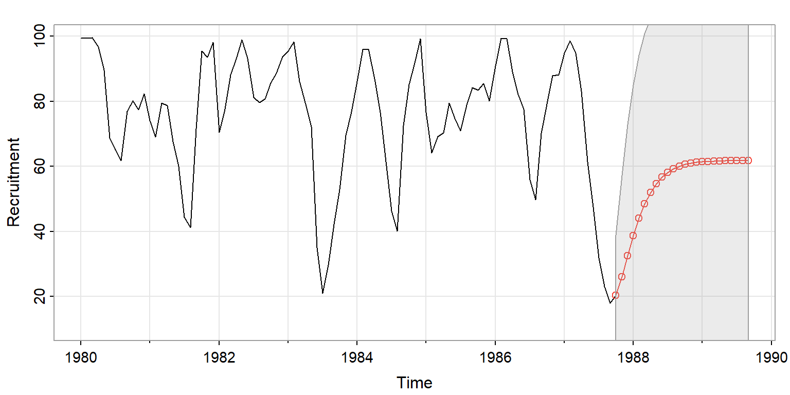
Figure 9: Recruitment: 24-month AR(2) forecast
The oscillatory forecast reflects the AR(2) structure; intervals widen with horizon.
Exponential Smoothing
Simple Exponential Smoothing
A widely used forecasting method:
\[\hat{X}(t+1) = \alpha X(t) + (1-\alpha) \hat{X}(t)\]
Equivalently: \[\hat{X}(t+1) = \hat{X}(t) + \alpha (X(t) - \hat{X}(t))\]
Interpretation: Update the forecast by a fraction \(\alpha\) of the most recent error.
EWMA and ARIMA Connection
Simple exponential smoothing is the optimal forecast for an ARIMA(0,1,1) model:
\[\nabla X(t) = W(t) - \lambda W(t-1)\]
where \(\alpha = 1 - \lambda\) is the smoothing parameter.
Key insight: Exponential smoothing is not just a heuristic—it has a solid statistical foundation.
Beyond Simple Smoothing
Holt-Winters methods extend exponential smoothing:
| Component | What it captures |
|---|---|
| Level \(\ell(t)\) | Local mean |
| Trend \(b(t)\) | Local slope |
| Season \(s(t)\) | Periodic pattern |
These ETS (Error-Trend-Seasonal) models form an alternative to SARIMA, widely used in business forecasting.
The Modeling Workflow
Identification → Estimation → Diagnostics
Iterate: If residuals show structure, refine the model and repeat.
Residual Diagnostics
After fitting, residuals should behave like white noise:
- ACF near zero at all lags
- No patterns in residual plot
- Ljung-Box test non-significant
Model Comparison
When multiple models seem plausible, use information criteria:
AIC (Akaike): \(-2\log L + 2k\)
BIC (Bayesian): \(-2\log L + k \log T\)
where \(k\) = number of parameters, \(T\) = sample size.
BIC penalizes complexity more heavily → favors simpler models.
Lower is better for both criteria.
Summary
Key Insights
- AR models: Current value depends on past values
- ACF decays; PACF cuts off at order \(p\)
- MA models: Current value depends on past shocks
- ACF cuts off at order \(q\); PACF decays
- ARIMA: Differencing handles non-stationarity
- The “I” integrates an ARMA process
- SARIMA: Captures seasonal patterns
- Combines regular and seasonal differencing
The Forecasting Reality
- Prediction intervals widen with forecast horizon
- Uncertainty grows; we cannot predict arbitrarily far ahead
- Exponential smoothing has ARIMA foundations
- EWMA is optimal for IMA(1,1)
- Model diagnostics are essential
- Residuals should be white noise
- Information criteria guide model selection
The Dual Aims, Revisited
Time domain methods emphasize prediction:
- Given the past, what comes next?
- How much uncertainty surrounds that forecast?
But prediction rests on understanding:
- The ACF/PACF patterns reveal the memory structure
- The model encodes why the past predicts the future
Next: Chapter 14 takes the complementary view—frequency domain methods reveal the periodic structure that drives the process.
Diagnostic Checklist
When building a time series forecast:
Plot the series: Identify trend, seasonality, variance changes
Transform if needed: Differencing, log transform
Examine ACF/PACF: Does PACF cut off? Does ACF cut off?
Fit candidate models: Start simple (AR or MA), add complexity if needed
Check residuals: ACF should be flat; Ljung-Box non-significant
Compare models: Use AIC/BIC for selection
Forecast with intervals: Report uncertainty honestly
Exercises
Team Exercise 1: AR(1) vs. MA(1) Signatures
Using stats::arima.sim():
- Generate 200 observations from AR(1) with \(\phi = 0.7\).
- Generate 200 observations from MA(1) with \(\theta = 0.7\).
- Plot the ACF and PACF for each. Can you tell them apart?
- Which cuts off sharply? Which decays exponentially?
Team Exercise 2: Model Selection
For the recruitment data (astsa::rec):
- Fit AR(1), AR(2), and AR(3) using
stats::ar.ols(). - Compare their AIC values.
- Does AIC agree with what the PACF suggests?
- What are the tradeoffs of parsimony vs. fit?
Team Exercise 3: Forecast Uncertainty
Using the global temperature series (astsa::gtemp_land):
- Fit an ARIMA model to the first differences.
- Generate a 20-year forecast with prediction intervals.
- Why do the intervals widen over time?
- What does this imply for long-range climate projection?
Discussion Questions
A model with great in-sample fit forecasts poorly. What went wrong?
When would you choose a simpler model despite higher AIC?
How do ARIMA models compare to machine learning for time series?